Applications of Engineering Seismology for Site Characterization

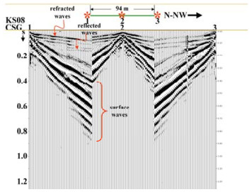
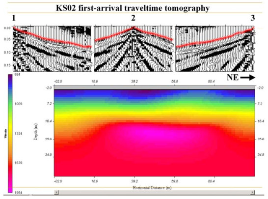
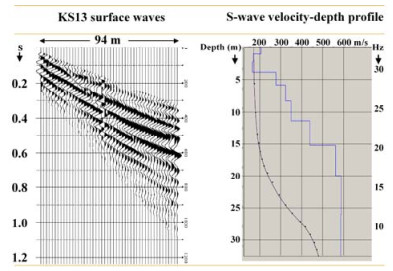
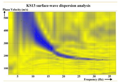
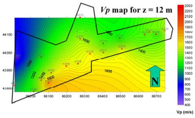
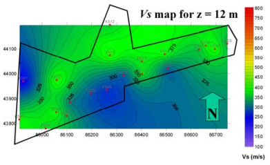
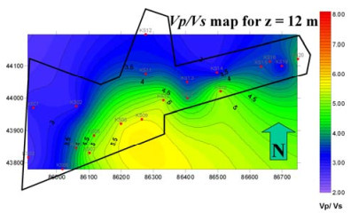
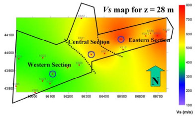
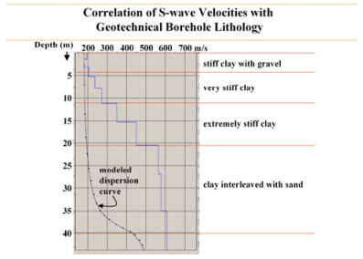
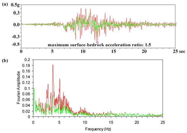
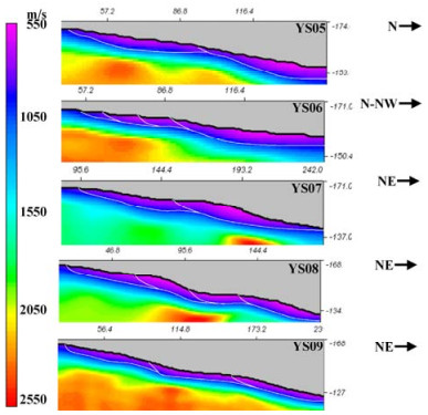
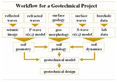
We determined the seismic model of the soil column within a residential project site in Istanbul, Turkey. Specifically, we conducted a refraction seismic survey at 20 locations using a receiver spread with 484.5-Hz vertical geophones at 2-m intervals. We applied nonlinear tomography to first-arrival times to estimate the P-wave velocity-depth profiles and performed Rayleigh-wave inversion to estimate the S-wave velocity-depth profiles down to a depth of 30 m at each of the locations. We then combined the seismic velocities with the geotechnical borehole information regarding the lithology of the soil column and determined the site-specific geotechnical earthquake engineering parameters for the site. Specifically, we computed the maximum soil amplification ratio, maximum surface-bedrock acceleration ratio, depth interval of significant acceleration, maximum soil-rock response ratio, and design spectrum periods TA-TB. We conducted reflection seismic surveys along five line traverses with lengths between 150 and 300 m and delineated landslide failure surfaces within the site. We recorded shot gathers at 2-m intervals along each of the seismic line traverses using a receiver spread with 4 840-Hz vertical geophones at 2-m intervals. We applied nonlinear tomography to first-arrival times to estimate a P-wave velocity-depth model and analyzed the reflected waves to obtain a seismic image of the deep near-surface along each of the line traverses.