Processing math: 100%
Advanced Search

Indexed by SCI、CA、РЖ、PA、CSA、ZR、etc .

Xuan Wang, Xinli Hu, Chang Liu, Lifei Niu, Peng Xia, Jian Wang, Jiehao Zhang. Research on Reservoir Landslide Thrust Based on Improved Morgenstern-Price Method. Journal of Earth Science, 2024, 35(4): 1263-1272. doi: 10.1007/s12583-021-1545-5
Citation: Xuan Wang, Xinli Hu, Chang Liu, Lifei Niu, Peng Xia, Jian Wang, Jiehao Zhang. Research on Reservoir Landslide Thrust Based on Improved Morgenstern-Price Method. Journal of Earth Science, 2024, 35(4): 1263-1272. doi: 10.1007/s12583-021-1545-5

Research on Reservoir Landslide Thrust Based on Improved Morgenstern-Price Method

doi: 10.1007/s12583-021-1545-5
More Information
  • Corresponding author: Xinli Hu, huxinli@cug.edu.cn
  • Received Date: 13 Jun 2021
  • Accepted Date: 10 Sep 2021
  • Available Online: 16 Aug 2024
  • Issue Publish Date: 30 Aug 2024
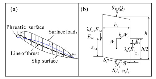
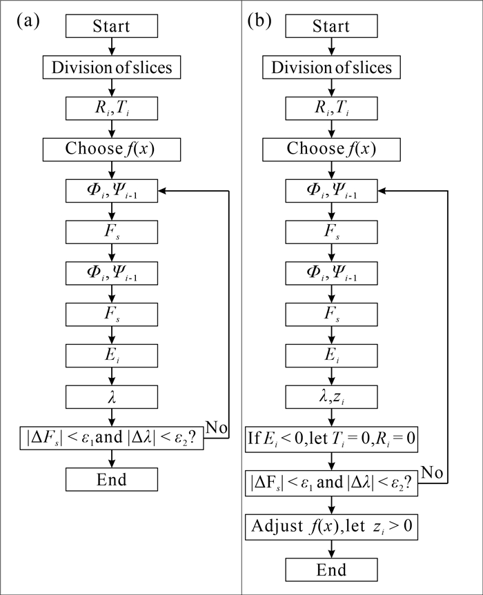
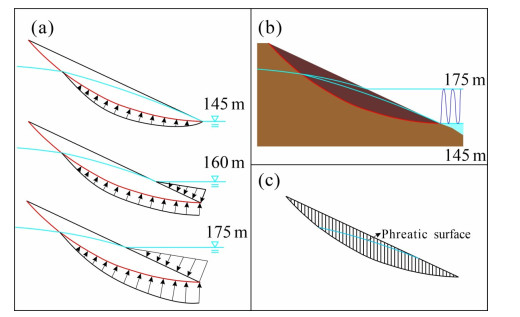
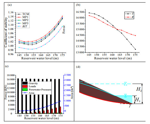
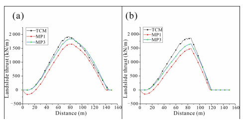
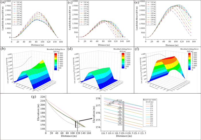
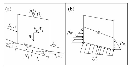
  • The curve of landslide thrust plays a key role in landslide design. The commonly used transfer coefficient method (TCM) and Morgenstern-Price method (MPM) are analyzed. TCM does not take into account the moment balance between slices. Although MPM considers the moment balance, the calculation is complex, and it does not consider that the force between slices may be less than zero at the back edge of the landslide. The rationality and feasibility of the improved MPM are verified by calculating the landslide stability coefficient and landslide thrust at different reservoir water levels. This paper studies the law of landslide thrust when the reservoir water level changes, and discusses the determination of design thrust, to provide a certain theoretical basis for the design of reservoir landslides.


  • APPENDIX
    Those important symbols used in this paper are listed alphabetically as follows.
    bi width if slice (m);
    ci cohesion (kPa);
    Ei interslice force (kN/m);
    fi a predefined function;
    Fs stability coefficient;
    hi center height of slice (m);
    kc influence coefficient of the earthquake;
    li length of sliding surface (m);
    Mi the moment of interslice force on the center of the bottom of a slice (kN/m);
    MPWi the moment of lateral water pressure on the center of the bottom of a slice (kN/m);
    MQi the moment of external load on the center of the bottom of a slice (kN/m);
    MUi the moment of buoyancy force on the center of the bottom of a slice (kN/m);
    Pwi lateral water pressure (kN);
    Qi external load (kN);
    Ri resistance (kN);
    Ti sliding force (kN);
    Ui buoyancy force (kN);
    Wi weight of slice (kN);
    zi the vertical height between interslice force and the bottom of a slice (m);
    αi the angle between the sliding surface and the horizontal direction (°);
    βi the angle between the water level line and the horizontal direction (°);
    γi the angle between the slope surface and the horizontal direction (°);
    θi the angle between the external load and the vertical direction (°);
    λ a constant arbitrarily chosen;
    φi friction angle (°);
    Φi transfer coefficient;
    Ψi transfer coefficient.
    Conflict of Interest
    The authors declare that they have no conflict of interest.
  • Landslide thrust, which could also be called the residual sliding force, refers to the sliding force before reinforcement in which the safety coefficient used is the current stability coefficient. The curve of landslide thrust can be used for parameter inversion, selection of anti-slide structure, and calculation of internal force of anti-slide structure. Landslide thrust not only affects the scale but also the cost and effect of the treatment project, so it plays a significant role in the process of landslide design. Generally, the calculation of stability coefficient and landslide thrust in the limit equilibrium method (LEM) can be divided into two methods, the non-strict slice method and the strict slice method. The former mainly includes the Swedish method (Fellenius, 1936), the simplified Bishop method (Bishop, 1955), and the residual thrust method (or transfer coefficient method, GB 50330-2013, 2013), while the latter mainly includes Spencer method (Spencer, 1967) and Morgenstern-Price method (Morgenstern and Price, 1965). Among them, the transfer coefficient method (TCM) and Morgenstern-Price method (MPM) are the two most widely used methods. The former has a simple calculation process, while the latter takes both static balance and moment balance into account but has more iterations.

    Zhou et al. (2014) compared TCM and the finite element strength reduction method to calculate the post thrust of a landslide anti-slide pile in the Three Gorges Reservoir area (TGRA) at different water levels. Due to the consideration of the water seepage force between slices, the post thrust calculated by the limit equilibrium method is slightly greater than that calculated by the finite element strength reduction method. Guo et al. (2020) introduced the complete finite element analysis into the limit equilibrium analysis, improved the vector summation method, and used the principle of minimum potential energy to determine the overall sliding direction of the landslide, which is more reasonable than the local sliding direction based on TCM. Zhang et al. (2021) used TCM to calculate the residual sliding force of the Shiliushubao landslide under the change of reservoir water level, determined the main control factors of slope cutting, and optimized the slope cutting scheme based on the artificial neural network algorithm, which not only reduced the cost but also improved the reliability.

    Morgenstern and Price (1965, 1967) assumed that the ratio of vertical tangential force to horizontal thrust between slices was a specific function, and established all static equilibrium equations for the first time, including force balance and moment balance. The solution idea of differential equation based on the Newton-Raphon method was described in detail and used in a digital computer program. Chen and Morgenstern (1983) improved MPM and proposed an integral method based on the geometric shape and physical characteristics of the slope. The solution of the balance equation was found through the assumed function, and the sensitivity of the assumed function to the balance equation was analyzed, to make the iteration more effective. Zhu et al. (2001, 2005) derived a concise recursive relation of adjacent slices when the force balance and moment balance were satisfied, proposed the selection of safety factor and initial value of scale parameter, simplified the numerical calculation program, and demonstrated the effectiveness and fast convergence by examples. To solve the two highly nonlinear equations of safety factor and scale function, Zhu and Lee (2002) proposed an alternative method to derive three equilibrium equations (horizontal force, vertical force, and moment) based on the assumption of normal stress distribution on the slip surface. Stolle and Guo (2008) proposed a simplified rigid finite element method considering the asymptotic yield of sliding, to eliminate the requirement of providing a constraint equation for the variation of interlayer forces in MPM. Sun et al. (2016a) combined with the numerical stability of global analysis and the flexibility of MPM, developed a general program for slope stability analysis and applied it to the study of stability evolution law of large-scale landslides. Deng et al. (2020) introduced the nonlinear model of shear stress and shear displacement and obtained double solutions of slope stress and displacement based on the extended MPM coupling force and displacement. In addition, MPM is also extended from 2D to 3D slope stability analysis (Sun et al., 2016b; Zheng, 2012; Cheng and Yip, 2007).

    With the rapid development of computer technology, a variety of optimization algorithms combined with MPM have been mined to solve the optimal slip surface and stability coefficient, which mainly included genetic algorithm (Zolfaghari et al., 2005), ant colony optimization algorithm (Kahatadeniya et al., 2009), support vector machine algorithm (Chen et al., 2011), hybrid particle swarm optimization algorithm (Khajehzadeh et al., 2012a, 2011), modified gravitational search algorithm (Khajehzadeh et al., 2012b), swarm intelligence algorithm (Gandomi et al., 2015), immune evolutionary optimization algorithm (Gao, 2015), imperialist competitive algorithm (Kashani et al., 2016), evolutionary optimization algorithm (Gandomi et al., 2017), improved whale optimization algorithm (Li et al., 2020) and so on.

    The researches above mainly focus on the overall stability analysis of landslides and the solution of the equilibrium equations. The solution of various optimization algorithms is mainly based on the principle of MPM. These methods are unique and effective, but there is a lack of research on the basic principle of MPM and it is difficult for general geotechnical engineers to master. Based on the analysis of TCM and MPM, this paper revises MPM based on TCM and verifies the rationality of the modification through an example. Furthermore, this paper also studies the landslide thrust under the change of reservoir water level, to provide some theoretical basis for the design of reservoir landslide.

    According to the longitudinal profile shape of the slip surface, the sliding body was divided into several numerical slices with unit width, regardless of the friction and tension between the slices.

    Considering the force equilibrium of slice i (Figure 1), resolving perpendicular to the slip surface,

    Ni=WicosαikcWisinαi+Qicos(θiαi)(PWi1PWi)sinαiUi+Ei1sin(αi1αi)
    (1)
    Figure  1.  Force analysis of slice (a) and water pressure at the boundary (b).

    and resolving parallel to the slip surface,

    Ei+Nitanφi+cili=Wisinαi+kcWicosαQisin(θiαi)+(PWi1PWi)cosαi+Ei1cos(αi1αi)
    (2)

    Substituting Eq.(1) into Eq.(2), resolving residual sliding force of slice i,

    Ei=Wisinαi+kcWicosαiQisin(θiαi)+(PWi1PWi)cosαi+Ei1cos(αi1αi){[WicosαkcWisinαi+Qicos(θiαi)(PWi1PWi)sinαiUi+Ei1sin(αi1αi)]tanφi+cili}/Fs=Wisinαi+kcWicosαiQisin(θiαi)+(PWi1PWi)cosαi{[WicosαkcWisinαi+Qicos(θiαi)(PWi1PWi)sinαiUi]tanφi+cili}/Fs+Ei1[cos(αi1αi)sin(αi1αi)tanφi/Fs]=TiRi/Fs+Ei1ψi1
    (3)

    in which

    Ti=Wisinαi+kcWicosαiQisin(θiαi)+(PWi1PWi)cosαi
    (4)
    Ri=[WicosαkcWisinαi+Qicos(θiαi)(PWi1PWi)sinαiUi]tanφi+cili
    (5)

    When calculating the global stability coefficient, we first assume an F0, put it in the position of Fs in the formula, and iterate to get En. If En > 0, it indicates that F0 is large, then we take F1 < F0 and calculate En. If En < 0, it indicates that F1 is small, F1 < F2 < F0 is taken until En ≈ 0, then Fn is the overall stability coefficient. It should be noted that when Ei is less than 0, we take Ei as equal to 0.

    Considering the force equilibrium of slice i (Figure 2), resolving perpendicular to the slip surface,

    Ni=(Wi+λfi1Ei1λfiEi+Qicosθi)cosαi+(EiEi1kcWi+Qisinθi)sinαiUi
    (6)
    Figure  2.  Diagram of landslide (a) and a typical slice (b).

    and resolving parallel to the slip surface,

    (Nitanφi+cili)/Fs=(Wi+λfi1Ei1λfiEi+Qicosθi)sinαi(EiEi1kcWi+Qisinθi)cosαi
    (7)

    Substituting Eq.(6) into Eq.(7),

    Ei[(sinαiλficosαi)tanφi+(cosαi+λfisinαi)Fs]=Ei1[(sinαiλfi1cosαi)tanφi+(cosαi+λfi1sinαi)Fs]+FsTiRiFs
    (8)

    It can be also written as

    EiΦi=ψi1Ei1Φi+FsTiRi
    (9)

    in which

    Ti=Wisinαi+kcWicosαiQisin(θiαi)
    (10)
    Ri=[WicosαkcWisinαi+Qicos(θiαi)Ui]tanφi+cili
    (11)
    Φi=(sinαiλficosαi)tanφi+(cosαi+λfisinαi)Fs
    (12)
    Φi1=(sinαi1λfi1cosαi1)tanφi1+(cosαi1+λfi1sinαi1)Fs
    (13)
    ψi1=(sinαiλfi1cosαi)tanφi+(cosαi+λfi1sinαi)FsΦi1
    (14)

    According to the end conditions, E0 = 0 and En = 0, the expression of stability coefficient Fs is derived as

    Fs=n1i=1(Rin1j=1ψj)+Rnn1i=1(Tin1j=1ψj)+Tn
    (15)

    The equation above is implicit because the variable Fs appears on both sides of the equation, so it needs to be solved by iterative method.

    Considering the bending moment of slice i at the midpoint of the bottom,

    Ei(zibi2tanαi)=Ei1(zi+bi2tanαi)λbi2(fiEi+fi1Ei1)+kcWhi2Qisinθihi
    (16)

    in which Mi = Eizi, Mi-1 = Ei-1zi-1. Mi, Mi-1 are the inter-slices moment,

    Mi=Mi1λbi2(fiEi+fi1Ei1)+bi2(Ei+Ei1)tanαi+kcWhi2Qisinθihi
    (17)

    According to the end conditions, M0 = 0 and Mn = 0, the expression of scale factor λ is derived as

    λ=ni=1[bi(Ei+Ei1)tanαi+kcWhi2Qisinθihi]ni=1bi(fiEi+fi1Ei1)
    (18)

    Calculation process (Figure 3a):

    Figure  3.  Calculation process of MPM (a) and modified MPM (b).

    1. Divide the slices. In computer programming, it can be divided into more than 100 equal-width slices.

    2. Calculate the sliding force Ti and anti-sliding force Ri of each slice.

    3. Select the inter-slices function f(x). Spencer method, f(x) = 1; Morgenstern price method, it can be chosen as

    f(x)=sinμ[π(xaxb)v]
    (19)

    where a and b are the left and right transverse coordinates, μ = 0 5.0, ν = 0.5 2.0.

    4. Set the initial value of stability factor Fs and undetermined factor λ. To achieve the effective transmission of thrust, the following requirements should be met

    Fs>sinαiλficosαicosαi+λfisinαitanφi
    (20)

    It is generally advisable to take Fs = 1 and λ = 0 as the initial value.

    5. Calculate the transfer coefficient Φi, ψi-1.

    6. Calculate the improved stability factor Fs.

    7. Apply the improved Fs and recalculate Φi, ψi-1.

    8. Recalculate the stability factor Fs.

    9. Calculate the inter-slice thrust Ei.

    10. Calculate the improved undetermined coefficient λ.

    11. Repeat process 5-10 until Fs and λ converge to a predetermined range.

    The calculation process of TCM is simple and can be completed by simple iteration, but it does not take into account the moment balance between the slices. The force between the slices calculated by TCM is parallel to the bottom of the slice rather than in the horizontal direction. In the design of the anti-slide pile, the landslide thrust should be in the horizontal direction. Therefore, the rationality and accuracy of the landslide thrust calculated by TCM is lower than that calculated by MPM.

    The calculation process of MPM is a little complicated and the force arm could be modified. Considering the moment balance of all slices, the force between slices is calculated in the horizontal direction. However, the condition when Ei < 0 is ignored in the calculation of the stability coefficient. That is, there may be tensile stress between slices, which is inconsistent with the actual situation. To eliminate this effect, the sliding force Ti and resistance Ri, but not the interforce Ei, should be reset to 0. To make it better to serve the design of the anti-slide pile, the MPM needs to be further modified (Figure 3b).

    Considering the force equilibrium of slice i (Figure 4), resolving perpendicular to the slip surface,

    Ni=(Wi+λfi1Ei1λfiEi+Qicosθi)cosαi+(EiEi1kcWi+QisinθiPwi1+Pwi)sinαiUi
    (21)
    Figure  4.  Water pressure at the boundary of slice on water (a) and underwater (b).

    and resolving parallel to the slip surface,

    (Nitanφi+cili)/Fs=(Wi+λfi1Ei1λfiEi+Qicosθi)sinαi(EiEi1kcWi+QisinθiPwi1+Pwi)cosαi
    (22)

    Substituting Eq.(21) into Eq.(22), resolving the residual sliding force of slice i,

    Ei[(sinαiλficosαi)tanφi+(cosαi+λfisinαi)Fs]=Ei1[(sinαiλfi1cosαi)tanφi+(cosαi+λfi1sinαi)Fs]+FsTiRi
    (23)

    It can be also written as,

    EiΦi=ψi1Ei1Φi+FsTiRi
    (24)

    In which

    Ti=Wisinαi+kcWicosαi+(Pwi1Pwi)cosαiQisin(θiαi)
    (25)
    Ri=[WicosαikcWisinαi+Qicos(θiαi)(Pwi1Pwi)sinαiUi]tanφi+cili
    (26)

    When slice i is partially on water,

    Pwi1=12ρwglCE2cos2βi
    (27)
    MPwi1=Pwi1(13lCE+12lisinαi)
    (28)
    Pwi=12ρwglDF2cos2βi
    (29)
    MPwi=Pwi(13lDF12lisinαi)
    (30)
    Ui=12ρwg(lCE+lDF)licos2βi
    (31)
    MUi=(UiρwglCElicos2βi)li/6
    (32)
    Qi=0
    (33)
    MQi=0
    (34)

    When slice i is underwater,

    Pwi1=12ρwg(lCE+lCA)lAE
    (35)
    MPwi1=ρwglCAlAE(12lAE+12lisinαi)+(Pwi1ρwglCAlAE)(13lAE+12lisinαi)
    (36)
    Pwi=12ρwg(lDF+lDB)lBF
    (37)
    MPwi=ρwglDBlBF(12lBF12lisinαi)+(PwiρwglDBlBF)(13lBF12lisinαi)
    (38)
    Ui=12ρwg(lCE+lDF)li
    (39)
    MUi=(UiρwglCEli)li/6
    (40)
    Qi=12ρwg(lCA+lDB)lAB
    (41)
    MQi=ρwglCAlAB(hisinγi)+(QiρwglCAlAB)(hisinγilAB/6)
    (42)

    According to the end conditions, E0 = 0 and En = 0, the expression of stability coefficient Fs is derived as

    Fs=n1i=1(Rin1j=1ψj)+Rnn1i=1(Tin1j=1ψj)+Tn
    (43)

    The equation above is implicit because the variable Fs appears on both sides of the equation, so it needs to be solved by iterative method.

    Considering the bending moment slice i at the midpoint of the bottom,

    Ei(zibi2tanαi)=Ei1(zi+bi2tanαi)λbi2(fiEi+fi1Ei1)+kcWihi2+MPwi1MPwiMUiMQi
    (44)

    in which Mi = Eizi and Mi-1 = Ei-1zi-1. Mi, Mi-1 are the inter-slices moment,

    Mi=Mi1λbi2(fiEi+fi1Ei1)+bi2(Ei+Ei1)tanαi+kcWihi2+MPwi1MPwiMUiMQi
    (45)

    According to the end conditions, M0=0 and Mn=0, the expression of scale factor λ is derived as

    λ=ni=1[bi(Ei+Ei1)tanαi+kcWihi+2(MPwi1MPwi)2MUi2MQi]ni=1bi(fiEi+fi1Ei1)
    (46)

    Calculation process:

    19. Do the same as MPM.

    10. Calculate the improved undetermined coefficient λ, zi.

    11. Take Ti = 0, Ri = 0 if Ei < 0.

    12. Repeat process 510 until Fs and λ converge to a predetermined range.

    13. Adjust f(x) to make zi ≥ 0.

    The generalized model of reservoir landslide is established as shown in Figure 5, and the physical and mechanical parameters of the main components of the landslide are shown in Table 1. Different methods are used to calculate the landslide stability coefficient and landslide thrust. Through an in-depth analysis of the calculation results, the rationality and feasibility of the improved MPM will be confirmed.

    Figure  5.  Hydraulic conditions of landslides at different reservoir water levels (a), diagram (b), and division of the landslide (c).
    Table  1.  Physical and mechanical parameters of landslide
    Nature Saturated
    γ (kN·m3) C (kPa) φ (º) γ (kN·m3) C (kPa) φ (º)
    Sliding mass 20 22
    Sliding belt 28 26 25 23
     | Show Table
    DownLoad: CSV

    For the convenience of narration, the original MPM is referred to as MP1, MP2 is used for modification of force arm, and MP3 for both force arm and Ei.

    Considering the balance of vertical force and moment between slices, the stability coefficient calculated by MP1 is higher than that of TCM under the same water level condition. But compared with the geological analysis, the ordinary method produces a great deviation (Hu et al., 2012). Due to absorbing the characteristics of both TCM and MPM, the stability coefficients calculated by MP2 and MP3 are both in the middle. Whether the force arm is modified or not, it still has a weak effect on the calculation results (Figure 6a). The modified one is slightly greater than that of the unmodified one. The rise in water level means the increase of external load, which can be found from the stability calculation formula that it is beneficial to the stability of the slope (Bi et al., 2012; Zhang et al., 2010). Therefore, the stability coefficient of the slope is rising in a straight line theoretically. However, from the calculation results, the stability coefficient calculated by different methods is basically the same, that is, the stability coefficient reduced first and then increased (Figure 6a).

    Figure  6.  Variation of stability coefficient (a), sliding force and resistance totally (b), sliding force only (c); Diagram of reservoir landslide (d).

    The stability coefficient is related to the sliding force and resistance of landslides. Dividing the total resistance by sliding force, it is not difficult to find that the change rule of its magnitude is the same as the stability coefficient (Figure 6a). With the increase of water level, the total resistance decreases in a straight line, while the total sliding force decreases in a quadratic way (Figure 6b). As the reservoir water level rises, the change of gravity and water pressure is gentle, while the external load rises quadratically (Figure 6c). This is because the external load, Q, is positively related to the area water acting on the slope. As the reservoir water level rises in a straight line, the area increases quadratically because of the inclination of the slope (Figure 6d and Eq. 47). Both the sliding force and resistance are affected by the rising water level, but the former is more sensitive and decreases faster, so the stability coefficient of slope descends first and then increases.

    ΔQ=12ρwgH2H2sinγ12ρwgH1H1sinγ=12ρwgH22H12sinγ
    (47)

    The stability coefficients calculated by MP2 are very little apart from MP3, so they can be dropped. For now, only TCM, MP1, and MP3 are considered. As shown in Figure 7, the landslide thrust under high and low water levels are calculated and drawn (safety factor is taken as 1.00). It can be seen from the figure that the change in the landslide thrust curve under the three methods is roughly the same. The landslide thrust curve obtained by MP3 is between TCM and MP1. However, the landslide thrust curves of MP1 and MP3 are smoother than that of TCM. This is because Ei calculated by MP is horizontal, while by TCM, Ei is parallel to the bottom of the slice, which will fluctuate due to the difference of slice dip angle α. Due to the consideration of the vertical forces between the slices, the landslide thrust calculated by MPM is closer to the real value. The maximum landslide thrust is 500 kN/m smaller than that calculated by TCM, which can save a lot of cost for the design of reinforcement. Compared with MP1, MP3 has modified the arm of force and considered the inter-slice force at the trailing edge of the landslide. As a result, MP3 is more reasonable and feasible.

    Figure  7.  Landslide thrust curve when the reservoir water level is 145 m (a) and 175 m (b).

    The current stability coefficient Fs0 was calculated first. In Eq.(26), Fs is taken at 1.00, Fs0, and 1.15 respectively, and the landslide thrust curve of slope under each water level is drawn (Figures 8a8f). Fs of 1.00 represents the current landslide thrust, Fs0 represents ultimate state, and 1.15 represents design condition which is related to the grade of slope.

    Figure  8.  Variations of landslide thrust with different safety factor: Fs = Fs0 (a) (b), Fs = 1.00 (c) (d) and Fs = 1.15 (e) (f), line of thrust when Fs = Fs0 (g).

    With the rise of water level, when Fs is taken Fs0, the position of the maximum thrust moves inward, and the overall landslide thrust decreases first and then increases. When Fs is taken at 1.00 and 1.15, the position of the maximum thrust moves inward, and the overall landslide thrust shows a decreasing trend. When Fs is set at the same value, the external load increases, which is conducive to the stability of the landslide and reduces the inter-slice force. When Fs is set at different values, due to the rise of water level, the larger the stability coefficient has been calculated, the more stable the slope is. To reach the ultimate equilibrium state, the inter-slice force should be greater.

    With the increase of water level, the thrust curve shows a trend of first outward and then inward (Figure 8g). The further out the line of thrust goes, the lower the slope stability is. At the time the reservoir water level is 154 m, and the stability coefficient is the lowest of 1.008.

    According to the shape of the slope, the position of the anti-slide pile is selected to determine the design thrust. Considering the resistance of soil in front of the pile, the thrust difference of pile position is generally taken as the design thrust. We have two options, one is 1.15–1.00, and the other is 1.15–Fs. At the pile location, the former design thrust is about 2 300 kN/m, while the latter is about 2 100 kN/m (Table 2). Considering the length and number of piles will have a great impact on the cost. The anti-slide pile resists the forward sliding of the soil at the back edge and prevents the rock and soil mass of the slope from the natural state to the limited equilibrium state. Design safety and pile-soil interaction have been already considered when 1.15 is taken, so the second scheme is not only feasible but also more economical.

    Table  2.  Thrust difference at different water levels
    Water level (m) Thrust difference (kN/m)
    1.15–1.00 1.15–Fs
    145 2 220.97 1 996.83
    148 2 279.44 2 066.51
    151 2 222.06 2 105.71
    154 2 209.82 2 091.64
    157 2 186.98 2 002.62
    160 2 123.97 1 773.28
    163 2 039.02 1 524.51
    166 1 945.68 1 238.94
    169 1 821.80 848.62
    172 1 718.89 516.65
    175 1 617.02 181.32
     | Show Table
    DownLoad: CSV

    The design of reservoir landslide still follows the general landslide, but the determination of reservoir landslide thrust lacks systematicness because of the complex hydrogeological environment and internal-external geological factors. In this paper, based on the analysis of TCM and MPM, MPM was revised to a certain extent. The force analysis was carried out on the reservoir landslide which can be significantly affected by the change of water level. The landslide thrust and design thrust were also studied and the following conclusions were drawn.

    1. The improved MPM combines the respective advantages of TCM and MPM. A small difference in stability coefficient will also lead to a large difference in landslide thrust. Through simple analysis of the stability coefficient and thrust curve with high and low water levels, the rationality of the improved MPM is confirmed.

    2. The landslide thrust under the natural state, limit equilibrium state, and design state under different reservoir water levels are studied. With the rise of reservoir water level, the overall landslide thrust and maximum value change obviously, and the law can be followed, but the universality of general landslide design is worth further studying.

    3. The stability of reservoir landslides is extremely sensitive to the reservoir water level. Accurate and timely access to groundwater level information is the key to the design of reservoir landslides. After the location of the pile is determined, the difference between the thrust in the design state and the limit equilibrium state can be chosen as the design thrust.

    The research on the post-thrust distribution of anti-slide piles in reservoir landslides based on the evolution model will be further carried out.

    ACKNOWLEDGMENTS: This study was supported by the Key Program of National Natural Science Foundation of China (No. 41630643), the National Key Research and Development Program of China (No. 2017YFC1501302), the Fundamental Research Funds for the Central Universities, China University of Geosciences (Wuhan) (No. CUGCJ1701), and the Science and Technology Projects of the Huaneng Lancang River Hydropower Co., Ltd. (No. HNKJ18-H24). The final publication is available at Springer via https://doi.org/10.1007/s12583-021-1545-5.
  • Bi, R. N., Ehret, D., Xiang, W., et al., 2012. Landslide Reliability Analysis Based on Transfer Coefficient Method: A Case Study from Three Gorges Reservoir. Journal of Earth Science, 23(2): 187–198. https://doi.org/10.1007/s12583-012-0244-7
    Bishop, A. W., 1955. The Use of the Slip Circle in the Stability Analysis of Slopes. Géotechnique, 5(1): 7–17. https://doi.org/10.1680/geot.1955.5.1.7
    Chen, C. F., Xiao, Z. Y., Zhang, G. B., 2011. Time-Variant Reliability Analysis of Three-Dimensional Slopes Based on Support Vector Machine Method. Journal of Central South University of Technology, 18(6): 2108–2114. https://doi.org/10.1007/s11771-011-0950-9
    Chen, Z. Y., Morgenstern, N. R., 1983. Extensions to the Generalized Method of Slices for Stability Analysis. Canadian Geotechnical Journal, 20(1): 104–119. https://doi.org/10.1139/t83-010
    Cheng, Y. M., Yip, C. J., 2007. Three-Dimensional Asymmetrical Slope Stability Analysis Extension of Bishop's, Janbu's, and Morgenstern–Price's Techniques. Journal of Geotechnical and Geoenvironmental Engineering, 133(12): 1544–1555. https://doi.org/10.1061/(asce)1090-0241(2007)133: 12(1544) doi: 10.1061/(asce)1090-0241(2007)133:12(1544
    Deng, D. P., Lu, K., Wen, S. S., et al., 2020. The Expanded LE Morgenstern-Price Method for Slope Stability Analysis Based on a Force-Displacement Coupled Mode. Geomechanics and Engineering, 23(4): 313–325. https://doi.org/10.12989/GAE.2020.23.4.313
    Fellenius, W., 1936. Calculation of the Stability of Earth Dams. Engineering, Environmental Science, 4: 445–463
    Gandomi, A. H., Kashani, A. R., Mousavi, M., et al., 2015. Slope Stability Analyzing Using Recent Swarm Intelligence Techniques. International Journal for Numerical and Analytical Methods in Geomechanics, 39(3): 295–309. https://doi.org/10.1002/nag.2308
    Gandomi, A. H., Kashani, A. R., Mousavi, M., et al., 2017. Slope Stability Analysis Using Evolutionary Optimization Techniques. International Journal for Numerical and Analytical Methods in Geomechanics, 41(2): 251–264. https://doi.org/10.1002/nag.2554
    Gao, W., 2015. Slope Stability Analysis Based on Immunised Evolutionary Programming. Environmental Earth Sciences, 74(4): 3357–3369. https://doi.org/10.1007/s12665-015-4372-0
    Guo, M. W., Liu, S. J., Wang, S. L., et al., 2020. Determination of Residual Thrust Force of Landslide Using Vector Sum Method. Journal of Engineering Mechanics, 146(7): 04020063. https://doi.org/10.1061/(asce)em.1943-7889.0001791
    Hu, X. L., Tang, H. M., Li, C. D., et al., 2012. Stability of Huangtupo Riverside Slumping Mass Ⅱ# under Water Level Fluctuation of Three Gorges Reservoir. Journal of Earth Science, 23(3): 326–334. https://doi.org/10.1007/s12583-012-0259-0
    Kahatadeniya, K. S., Nanakorn, P., Neaupane, K. M., 2009. Determination of the Critical Failure Surface for Slope Stability Analysis Using Ant Colony Optimization. Engineering Geology, 108(1/2): 133–141. https://doi.org/10.1016/j.enggeo.2009.06.010
    Kashani, A. R., Gandomi, A. H., Mousavi, M., 2016. Imperialistic Competitive Algorithm: A Metaheuristic Algorithm for Locating the Critical Slip Surface in 2-Dimensional Soil Slopes. Geoscience Frontiers, 7(1): 83–89. https://doi.org/10.1016/j.gsf.2014.11.005
    Khajehzadeh, M., Taha, M. R., El-Shafie, A., et al., 2012a. Locating the General Failure Surface of Earth Slope Using Particle Swarm Optimisation. Civil Engineering and Environmental Systems, 29(1): 41–57. https://doi.org/10.1080/10286608.2012.663356
    Khajehzadeh, M., Taha, M. R., El-Shafie, A., et al., 2012b. A Modified Gravitational Search Algorithm for Slope Stability Analysis. Engineering Applications of Artificial Intelligence, 25(8): 1589–1597. https://doi.org/10.1016/j.engappai.2012.01.011
    Khajehzadeh, M., Taha, M. R., El-Shafie, A., 2011. Reliability Analysis of Earth Slopes Using Hybrid Chaotic Particle Swarm Optimization. Journal of Central South University, 18(5): 1626–1637. https://doi.org/10.1007/s11771-011-0882-4
    Li, S. H., Wu, L. Z., Luo, X. H., 2020. A Novel Method for Locating the Critical Slip Surface of a Soil Slope. Engineering Applications of Artificial Intelligence, 94: 103733. https://doi.org/10.1016/j.engappai.2020.103733
    Morgenstern, N. R., Price, V. E., 1965. The Analysis of the Stability of General Slip Surfaces. Géotechnique, 15(1): 79–93. https://doi.org/10.1680/geot.1965.15.1.79
    Morgenstern, N. R., Price, V. E., 1967. A Numerical Method for Solving the Equations of Stability of General Slip Surfaces. The Computer Journal, 9(4): 388–393. https://doi.org/10.1093/comjnl/9.4.388
    GB 50330-2013, 2013. Technical Code for Building Slope Engineering. China Architecture and Building Press, Beijing (in Chinese)
    Spencer, E., 1967. A Method of Analysis of the Stability of Embankments Assuming Parallel Inter-Slice Forces. Géotechnique, 17(1): 11–26. https://doi.org/10.1680/geot.1967.17.1.11
    Stolle, D., Guo, P. J., 2008. Limit Equilibrium Slope Stability Analysis Using Rigid Finite Elements. Canadian Geotechnical Journal, 45(5): 653–662. https://doi.org/10.1139/t08-010
    Sun, G. H., Cheng, S. G., Jiang, W., et al., 2016a. A Global Procedure for Stability Analysis of Slopes Based on the Morgenstern-Price Assumption and Its Applications. Computers and Geotechnics, 80: 97–106. https://doi.org/10.1016/j.compgeo.2016.06.014
    Sun, G. H., Huang, Y. Y., Li, C. G., et al., 2016b. Formation Mechanism, Deformation Characteristics and Stability Analysis of Wujiang Landslide near Centianhe Reservoir Dam. Engineering Geology, 211: 27–38. https://doi.org/10.1016/j.enggeo.2016.06.025
    Zhang, T. T., Yan, E. C., Cheng, J. T., et al., 2010. Mechanism of Reservoir Water in the Deformation of Hefeng Landslide. Journal of Earth Science, 21(6): 870–875. https://doi.org/10.1007/s12583-010-0139-4
    Zhang, Z. H., Liu, W., Zhang, Y. B., et al., 2021. Towards on Slope-Cutting Scheme Optimization for Shiliushubao Landslide Exposed to Reservoir Water Level Fluctuations. Arabian Journal for Science and Engineering, 46(11): 10505–10517. https://doi.org/10.1007/s13369-021-05360-w
    Zheng, H., 2012. A Three-Dimensional Rigorous Method for Stability Analysis of Landslides. Engineering Geology, 145/146: 30–40. https://doi.org/10.1016/j.enggeo.2012.06.010
    Zhou, C. M., Shao, W., van Westen, C. J., 2014. Comparing Two Methods to Estimate Lateral Force Acting on Stabilizing Piles for a Landslide in the Three Gorges Reservoir, China. Engineering Geology, 173: 41–53. https://doi.org/10.1016/j.enggeo.2014.02.004
    Zhu, D. Y., Lee, C. F., 2002. Explicit Limit Equilibrium Solution for Slope Stability. International Journal for Numerical and Analytical Methods in Geomechanics, 26(15): 1573–1590. https://doi.org/10.1002/nag.260
    Zhu, D. Y., Lee, C. F., Qian, Q. H., et al., 2001. A New Procedure for Computing the Factor of Safety Using the Morgenstern-Price Method. Canadian Geotechnical Journal, 38(4): 882–888. https://doi.org/10.1139/cgj-38-4-882
    Zhu, D. Y., Lee, C. F., Qian, Q. H., et al., 2005. A Concise Algorithm for Computing the Factor of Safety Using the Morgenstern–Price Method. Canadian Geotechnical Journal, 42(1): 272–278. https://doi.org/10.1139/t04-072
    Zolfaghari, A. R., Heath, A. C., McCombie, P. F., 2005. Simple Genetic Algorithm Search for Critical Non-Circular Failure Surface in Slope Stability Analysis. Computers and Geotechnics, 32(3): 139–152. https://doi.org/10.1016/j.compgeo.2005.02.001
  • Relative Articles

    [1]Longqi Li, Yunhuang Yang, Tianzhi Zhou, Mengyun Wang. Data-Driven Combination-Interval Prediction for Landslide Displacement Based on Copula and VMD-WOA-KELM Method[J]. Journal of Earth Science, 2025, 36(1): 291-306. doi: 10.1007/s12583-021-1555-3
    [2]Jiefei Zhang, Shu Zhang, Huiming Tang, Qingbing Liu, Qiang Li, Huan Zhang. Creeping reservoir landslide progressive evolution process: from large-scale direct shear creep test to seepage-mechanical-deformation block model[J]. Journal of Earth Science. doi: 10.1007/s12583-025-0215-4
    [3]Guochao Fu, Hua Pan, Jiang Cheng. An Uncertainty Analysis of the Newmark Displacement Model for Earthquake-Induced Landslides in the Jiuzhaigou National Geopark[J]. Journal of Earth Science, 2024, 35(6): 1998-2012. doi: 10.1007/s12583-021-1519-7
    [4]Yiqiu Yan, Changbao Guo, Yanan Zhang, Zhendong Qiu, Caihong Li, Xue Li. Development and Deformation Characteristics of Large Ancient Landslides in the Intensely Hazardous Xiongba-Sela Section of the Jinsha River, Eastern Tibetan Plateau, China[J]. Journal of Earth Science, 2024, 35(3): 980-997. doi: 10.1007/s12583-023-1925-y
    [5]Hongfu Zhou, Fei Ye, Wenxi Fu, Bin Liu, Tian Fang, Rui Li. Dynamic Effect of Landslides Triggered by Earthquake: A Case Study in Moxi Town of Luding County, China[J]. Journal of Earth Science, 2024, 35(1): 221-234. doi: 10.1007/s12583-022-1806-y
    [6]Lu Guo, Keqiang He, Honghua Liu, Fandi Meng, Xuchun Wang. Physical Prediction Model of Compound Hydrodynamic Unload-Load Response Ratio and Its Application in Reservoir Colluvium Landslide[J]. Journal of Earth Science, 2024, 35(4): 1304-1315. doi: 10.1007/s12583-022-1662-9
    [7]Shilin Luo, Da Huang, Jianbing Peng, Zhouzhou Xie, Zhiyu Yang, Roberto Tomás. Insights into Reservoir-Triggered Landslides Development and Its Influence Factors in the Three Gorges Reservoir Area, China[J]. Journal of Earth Science, 2024, 35(6): 1979-1997. doi: 10.1007/s12583-024-0024-1
    [8]Qianyun Wang, Huiming Tang, Pengju An, Kun Fang, Junrong Zhang, Minghao Miao, Qingwen Tan, Lei Huang, Shengming Hu. Insight into the Permeability and Microstructure Evolution Mechanism of the Sliding Zone Soil: A Case Study from the Huangtupo Landslide, Three Gorges Reservoir, China[J]. Journal of Earth Science, 2024, 35(3): 941-954. doi: 10.1007/s12583-023-1828-0
    [9]Xianmin Wang, Jing Yin, Menghan Luo, Haifeng Ren, Jing Li, Lizhe Wang, Dongdong Li, Guojun Li. Active High-Locality Landslides in Mao County: Early Identification and Deformational Rules[J]. Journal of Earth Science, 2023, 34(5): 1596-1615. doi: 10.1007/s12583-021-1505-0
    [10]Defu Tong, Aijun Su, Fei Tan, Jiandong Tang, Xiongwei Yi. Genetic Mechanism of Water-Rich Landslide Considering Antecedent Rainfalls: A Case Study of Pingyikou Landslide in Three Gorges Reservoir Area[J]. Journal of Earth Science, 2023, 34(6): 1878-1891. doi: 10.1007/s12583-022-1722-1
    [11]Ning Zhu, Yingchang Cao, Kelai Xi, Songtao Wu, Rukai Zhu, Miaomiao Yan, Shunkang Ning. Multisourced CO2 Injection in Fan Delta Conglomerates and Its Influence on Reservoir Quality: Evidence from Carbonate Cements of the Baikouquan Formation of Mahu Sag, Junggar Basin, Northwestern China[J]. Journal of Earth Science, 2021, 32(4): 901-918. doi: 10.1007/s12583-020-1360-4
    [12]Entao Liu, Jian-Xin Zhao, Hua Wang, Songqi Pan, Yuexing Feng, Qianglu Chen, Faye Liu, Jiasheng Xu. LA-ICPMS in-situ U-Pb Geochronology of Low-Uranium Carbonate Minerals and Its Application to Reservoir Diagenetic Evolution Studies[J]. Journal of Earth Science, 2021, 32(4): 872-879. doi: 10.1007/s12583-020-1084-5
    [13]Dan Gao, Rihui Cheng, Yanjie Shen, Liaoliang Wang, Xiaoqiang Hu. Weathered and Volcanic Provenance-Sedimentary System and Its Influence on Reservoir Quality in the East of the Eastern Depression, the North Yellow Sea Basin[J]. Journal of Earth Science, 2018, 29(2): 353-368. doi: 10.1007/s12583-017-0945-z
    [14]Gang Rao, Yali Cheng, Aiming Lin, Bing Yan. Relationship between Landslides and Active Normal Faulting in the Epicentral Area of the AD 1556 M~8.5 Huaxian Earthquake, SE Weihe Graben (Central China)[J]. Journal of Earth Science, 2017, 28(3): 545-554. doi: 10.1007/s12583-017-0900-z
    [15]Renguang Zuo, Carranza Emmanuel John M.. A Fractal Measure of Spatial Association between Landslides and Conditioning Factors[J]. Journal of Earth Science, 2017, 28(4): 588-594. doi: 10.1007/s12583-017-0772-2
    [16]Huanqing Chen, Yo ng le Hu, Jiuqiang Jin, Qiquan Ran, Lin Yan. Fine Stratigraphic Division of Volcanic Reservoir by Uniting of Well Data and Seismic Data[J]. Journal of Earth Science, 2014, 25(2).
    [17]Chong Xu, Xiwei Xu, Fuchu Dai, Jianzhang Xiao, Xibin Tan, Renmao Yuan. Landslide Hazard Mapping Using GIS and Weight of Evidence Model in Qingshui River Watershed of 2008 Wenchuan Earthquake Struck Region[J]. Journal of Earth Science, 2012, 23(1): 97-120. doi: 10.1007/s12583-012-0236-7
    [18]earch on the Distribution of Major Metal Elements in the Typical Landslide Soil of the Three Gorges Reservoir Area[J]. Journal of Earth Science, 2012, 23(2). doi: 10.1007/s12583-012-0000-0
    [19]Renneng Bi, Dominik Ehret, Wei Xiang, Joachim Rohn, Markus Schleier, Jiwei Jiang. Landslide Reliability Analysis Based on Transfer Coefficient Method: A Case Study from Three Gorges Reservoir[J]. Journal of Earth Science, 2012, 23(2): 187-198. doi: 10.1007/s12583-012-0244-7
    [20]Dominik Ehret, Joachim Rohn, Christian Dumperth, Susan Eckstein, Stefanie Ernstberger, Karel OTTE, René Rudolph, Johannes Wiedenmann, Wei Xiang, Renneng Bi. Frequency Ratio Analysis of Mass Movements in the Xiangxi Catchment, Three Gorges Reservoir Area, China[J]. Journal of Earth Science, 2010, 21(6): 824-834. doi: 10.1007/s12583-010-0134-9
  • Created with Highcharts 5.0.7Amount of accessChart context menuAbstract Views, HTML Views, PDF Downloads StatisticsAbstract ViewsHTML ViewsPDF Downloads2024-062024-072024-082024-092024-102024-112024-122025-012025-022025-032025-042025-050102030405060
    Created with Highcharts 5.0.7Chart context menuAccess Class DistributionFULLTEXT: 29.7 %FULLTEXT: 29.7 %META: 29.7 %META: 29.7 %PDF: 40.5 %PDF: 40.5 %FULLTEXTMETAPDF
    Created with Highcharts 5.0.7Chart context menuAccess Area DistributionBrazil: 3.7 %Brazil: 3.7 %China: 17.5 %China: 17.5 %India: 1.9 %India: 1.9 %Norway: 3.7 %Norway: 3.7 %Reserved: 6.3 %Reserved: 6.3 %Russian Federation: 2.2 %Russian Federation: 2.2 %United States: 63.2 %United States: 63.2 %海得拉巴: 0.7 %海得拉巴: 0.7 %罗奥尔凯埃: 0.7 %罗奥尔凯埃: 0.7 %BrazilChinaIndiaNorwayReservedRussian FederationUnited States海得拉巴罗奥尔凯埃

Catalog

    通讯作者: 陈斌, bchen63@163.com
    • 1. 

      沈阳化工大学材料科学与工程学院 沈阳 110142

    1. 本站搜索
    2. 百度学术搜索
    3. 万方数据库搜索
    4. CNKI搜索

    Figures(8)  / Tables(2)

    Article Metrics

    Article views(78) PDF downloads(109) Cited by()
    Proportional views
    Related

    /

    DownLoad:  Full-Size Img  PowerPoint
    Return
    Return