Loading [MathJax]/jax/element/mml/optable/GreekAndCoptic.js
Advanced Search

Indexed by SCI、CA、РЖ、PA、CSA、ZR、etc .

Longqi Li, Yunhuang Yang, Tianzhi Zhou, Mengyun Wang. Data-Driven Combination-Interval Prediction for Landslide Displacement Based on Copula and VMD-WOA-KELM Method. Journal of Earth Science, 2025, 36(1): 291-306. doi: 10.1007/s12583-021-1555-3
Citation: Longqi Li, Yunhuang Yang, Tianzhi Zhou, Mengyun Wang. Data-Driven Combination-Interval Prediction for Landslide Displacement Based on Copula and VMD-WOA-KELM Method. Journal of Earth Science, 2025, 36(1): 291-306. doi: 10.1007/s12583-021-1555-3

Data-Driven Combination-Interval Prediction for Landslide Displacement Based on Copula and VMD-WOA-KELM Method

doi: 10.1007/s12583-021-1555-3
More Information
  • Corresponding author: Longqi Li, lilongqi2014@cdut.edu.cn
  • Received Date: 29 Jun 2021
  • Accepted Date: 26 Sep 2021
  • Available Online: 10 Feb 2025
  • Issue Publish Date: 28 Feb 2025
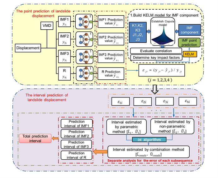
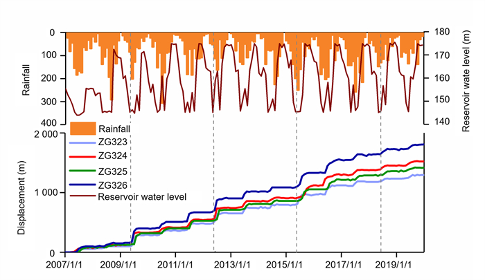
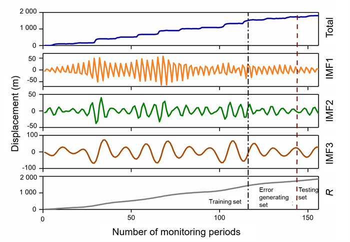
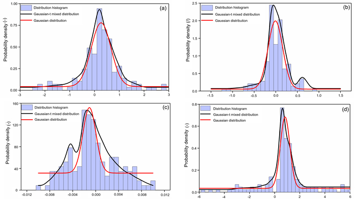
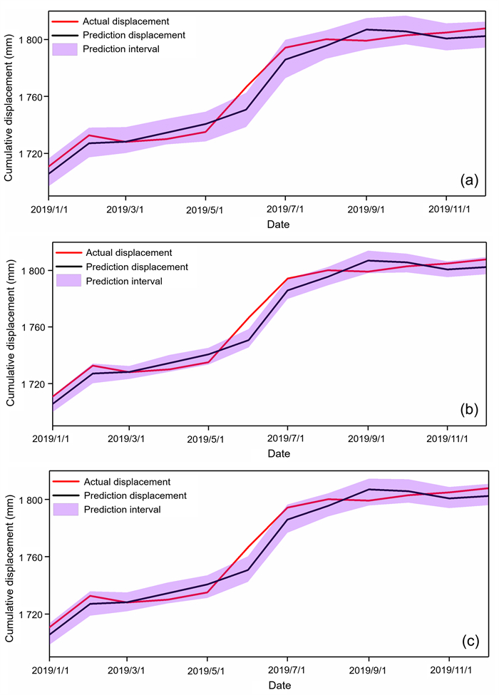
  • To tackle the difficulties of the point prediction in quantifying the reliability of landslide displacement prediction, a data-driven combination-interval prediction method (CIPM) based on copula and variational-mode-decomposition associated with kernel-based-extreme-learning-machine optimized by the whale optimization algorithm (VMD-WOA-KELM) is proposed in this paper. Firstly, the displacement is decomposed by VMD to three IMF components and a residual component of different fluctuation characteristics. The key impact factors of each IMF component are selected according to Copula model, and the corresponding WOA-KELM is established to conduct point prediction. Subsequently, the parametric method (PM) and non-parametric method (NPM) are used to estimate the prediction error probability density distribution (PDF) of each component, whose prediction interval (PI) under the 95% confidence level is also obtained. By means of the differential evolution algorithm (DE), a weighted combination model based on the PIs is built to construct the combination-interval (CI). Finally, the CIs of each component are added to generate the total PI. A comparative case study shows that the CIPM performs better in constructing landslide displacement PI with high performance.


  • Conflict of Interest
    The authors declare that they have no conflict of interest.
  • Landslide is a common natural disaster which poses a huge threat to human life and property (Liu et al., 2016; Li et al., 2010). Recently, thousands of landslides have occurred in the Three Gorges Reservoir in China, which are triggered by the strong rainfall and massive change of the reservoir water level (Ma et al., 2017; Zhou et al., 2016; Yin et al., 2010). A bunch of studies have been carried out on landslide prediction and treatment (Huang et al., 2017; Intrieri et al., 2013; Li et al., 2012). Thereinto, predicting landslide displacement reasonably is significant and essential for early warning of such hazard.

    The evolution of landslide is a nonlinear complex dynamic process, while the related deformation is usually affected by multiple factors, such as geological settings, external environment change and human activities, etc. Some scholars (Herrera et al., 2009; Corominas et al., 2005) have attempted to establish physical models by building the relationship between deformation and the physical parameters of geotechnical materials in some given area. Although the established model is physically straightforward, the values of the related physical parameters are usually hard to obtain and always change with the transformation of landslide mass, especially in some complex large landslides. Therefore, the so-called data-driven models have been put forward from the initial deterministic model to the disposition-time statistical analysis model, subsequently to the nonlinear machine learning model during recent years (Zhou et al., 2016; Lian et al., 2014; Yin and Yan, 1996; Saito, 1965). These models are mostly established based on the deformation monitoring data and the deformation-related impact factors. Compared with the physical model, the data required by the data-driven model is easier to obtain. Nevertheless, the frequently-used statistical analysis model, nonlinear regression or polynomial fitting methods have been verified to be hard to perform deformation prediction efficiently. More recently, a number of scholars have resorted to the signal decomposition techniques (for instance, the empirical mode decomposition (EMD), the ensemble empirical mode decomposition (EEMD), the complete ensemble empirical mode decomposition with adaptive noise (CEEMDAN)) (Li L Q et al., 2021; Deng et al., 2017; Lin et al., 2011), combining with machine learning methods (for instance, the support vector machine (SVM), the extreme learning machine (ELM), the artificial neural network (ANN)) (Cao et al., 2016; Du et al., 2013; Liu et al., 2016; Wu et al., 2016; Zhou et al., 2016; Lian et al., 2014), to deal with this problem. In this measure, the landslide displacement is decomposed into a series of components with different characteristics, whose predicted values obtained by the machine learning models are added together to get the total predicted value. Compared with the traditional statistical prediction method, this measure has been verified to have a higher prediction accuracy and stronger generalization ability. However, the above studies mostly focus on the deterministic point prediction, and did not consider how to evaluate the uncertainties exist in the prediction process and quantify the reliability of the predicted result. For a complex dynamic landslide system, there are a variety of uncertainties involving the geological settings, measurement technology and prediction model exist during the displacement prediction process (Phoon and Kulhawy, 1999a, b), which can be quantified by constructing a PI (Wan et al., 2014). In recent years, although interval prediction has been widely applied in different fields (Lins et al., 2015; Shrivastava and Panigrahi, 2013; Khosravi et al., 2010; Shrestha and Solomatine, 2006), there is only a little work focusing on the landslide displacement PI. For instance, Wang et al. (2019) used the PSO-ELM of two-node output layer to directly obtain the upper and lower limits of the PI. Ma et al. (2018) adopted the Bootstrap combining with machine learning method to calculate the system error and random error caused by the uncertainties during constructing the PI. However, the former has a relatively low stability and higher calculation cost, while the latter has a higher requirement for parameter selection. Once the parameters fall into the local optimum during the calculation process, the prediction accuracy will be greatly reduced.

    In this paper, we propose a combination-interval prediction method based on Copula and VMD-WOA-KELM model to construct the PI. Firstly, the real monitoring displacement is decomposed by VMD to some displacement components, whose key impact factors are respectively determined by establishing their individual Copula model. The WOA-KELM model of each displacement component is then built using these key impact factors to conduct the dynamic point prediction. The point prediction error of each displacement component is calculated simultaneously. By comparing the error fitting degrees of the PDFs fitted by Gaussian distribution and Gaussian-t mixture distribution for each displacement component, whose optimum prior distribution form can be selected according to the highest fitting degree to construct the parametric-method-based PI. On the other hand, the optimal window width kernel density estimation is used to obtain the PDF of the prediction error for each displacement component, further to construct the non-parametric-method-based PI. Finally, we combine the PIs of each displacement component calculated by the above two methods through DE to fulfill the better performance. The PI of total displacement is finally obtained by superimposing the PI of each displacement component.

    The VMD is a new adaptive signal decomposition algorithm proposed by Dragomiretskiy and Zosso (2014). It can decompose the complex non-stationary signal into different modal component μ_k with its central frequency. It can not only effectively overcome the modal aliasing phenomenon exist in the EMD process, but also deal with the endpoint effect through mirroring continuation, and filter out the noise while retain the useful components in the original signal (Li et al., 2018; Xu and Niu, 2018).

    The occurrence of landslides is usually accompanied by abrupt displacement variation. If the original displacement data sequence is directly used in displacement prediction, the trained model may misidentify the abrupt segment as abnormal data (Li et al., 2019) to increase difficulties of displacement prediction. Meantime, estimating error at the first sharp point according to the prediction error PDF in the earlier stable deformation stage will result a great result bias, and the poor point prediction effect at this point will lead to an error spurt, which may result in accumulated effect to the prediction error estimation for the following point and reduce reliability of the interval prediction model. We use the VMD to decompose displacement into a series of displacement component to extract the displacement local features. The prediction error PDF of each displacement component is relatively stable, and the work mainly focuses on how to find the specific error PDF for each component, which can be used to estimate their error at the next point effectively.

    Selecting the effective input data can improve the prediction accuracy and give full play to the prediction performance of the model, which usually relies on evaluating the correlation between the input and output data correctly. The traditional linear correlation analysis has limitations for random variables that satisfy the non-normal distribution characteristic, which is difficult to deal with the variables with "thick tails". The coupla method gives a new insight to cope with this problem. Sklar (1996) suggested that for multiple marginal distribution functions $ {\mathrm{F}}_{1}\left({x}_{1}\right), {\mathrm{F}}_{2}\left({x}_{2}\right), ..., {\mathrm{F}}_{\mathrm{N}}\left({x}_{N}\right) $, there is a copula function C that satisfies the following formula.

    F(x1,x2,...,xN)=C(F1(x1),F2(x2),...,FN(xN)) (1)

    where, $ \mathrm{F}({x}_{1}, {x}_{2}, ..., {x}_{N}) $ is the joint distribution function of the marginal distribution $ {\mathrm{F}}_{1}\left({x}_{1}\right), {\mathrm{F}}_{2}\left({x}_{2}\right), ..., {\mathrm{F}}_{\mathrm{N}}\left({x}_{N}\right) $.

    Typical copula functions are mainly categorized into two groups (Reboredo, 2011). One is the elliptic copula function including Gaussian copula and Student t copula. The other is the Archimedes copula function including Gumbel copula, Clayton copula, and Frank copula. In practical application, the optimal copula function for target data is usually determined by Akaike information criterion (AIC) and Bayesian information criterion (BIC) (Gao, 2019; Posada and Buckley, 2004).

    L=1nni=1(peipi)2 (2)
    AIC=2ln(L)+2m (3)
    BIC=2ln(L)+mln(n) (4)

    where $ p{\mathrm{e}}_{i} $ is the empirical probability; $ {p}_{i} $ is the theoretic frequency; m is the number of the model parameter; n is the number of data samples, and L is the maximum log-likelihood function. In this study, we choose the copula function with the minimum AIC and BIC values as the optimal function.

    The correlation between the impact factors and displacement can be evaluated by the Kendall rank correlation coefficient τ and the upper tail correlation coefficient. When their values are larger than 0.6, there is a strong correlation between the two variables (Liao et al., 2019; Deng et al., 2017). The detailed calculation process can refer to the literature by Tang (2018).

    According to the previous study (Sebbar et al., 2020), compared with the traditional neural network and SVM methods, the kernel extreme learning machine (KELM), which is an optimized method of the ELM, can effectively save the training time and avoid the overfitting as well as the local optimum problems through reducing the number of relative parameters. The ELM is a feedforward neural network training model with maximum likelihood of single hidden layer, which has great generalization ability and fast learning speed (Huang et al., 2006a, b; Huang, 2003). The basic network structure is shown in Figure 1.

    Figure  1.  KELM network structure diagram

    For sample $ ({x}_{i}, {y}_{i}) $, $ {x}_{i}=[{x}_{i1}, {x}_{i2}, ..., {x}_{im}{]}^{T}\in {R}^{m} $, $ {y}_{i}\in R $, the output value of ELM is expressed as follows.

    f(x)=Ni=1βih(ωixi+bi) (5)

    where N is the number of hidden node; $ {\beta }_{i}=[{\beta }_{1}, {\beta }_{2}, ..., {\beta }_{N}] $ is the weight vector connecting the ith hidden node and the output nodes; $ {\omega }_{i}=[{\omega }_{1i}, {\omega }_{2i}, ..., {\omega }_{mi}] $ is the weight vector connecting the ith hidden node and input nodes; $ {b}_{i}=[{b}_{1}, {b}_{2}, ..., {b}_{2}] $ is the threshold of the ith hidden node; $ h({\omega }_{i}\cdot {x}_{i}+{b}_{i}) $ is the output function of the hidden node. The training goal of ELM is to calculate the output weight matrix $ \beta $ that can achieve the best prediction effect. This training process can be fulfilled by least square linear regression using the hidden layer output matrix and real output data to implement. The least square solution $ \stackrel{-}{\beta } $ is shown in Eq. (6).

    β=H+Y (6)

    where $ {H}^{+} $ is the Moore-Penrose generalized inverse matrix of the hidden layer output matrix H.

    H=[h(ω11xi1+b1)h(ω1NxiN+bN)h(ωm1xim+b1)h(ωmNxiN+bN)] (7)

    To improve generalization ability and stability of ELM algorithm, Huang et al. (2012) introduced the kernel function into the ELM to form the KELM. Based on the orthogonal projection method and ridge regression theory, the value of $ \beta $ can be calculated by adding the coefficient 1/C. The calculation formula is expressed as follows.

    β=HT(1C+HHT)1Y (8)

    Therefore, the output function of ELM is expressed as follows.

    f(x)=h(x)HT(1C+HHT)1T (9)

    The kernel function is used instead of H(x), and the output function of KELM is expressed as follows.

    f(x)=[K(x,x1)K(x,xN)]T(1C+HHT)1T (10)

    Herein, we select the most widely used radial basis function as the kernel function $ K(x, {x}_{i}) $ of the KELM algorithm.

    K(x,xi)=exp(λxxi2) (11)

    where $ \lambda $ is the kernel function parameter, and $ {\lambda }_{0} $; $ {‖x-{x}_{i}‖}^{2} $ is the square Euclidean distance between input feature vector $ x $ and $ {x}_{i} $.

    In this study, we take the whale optimization algorithm (WOA) to optimize the penalty coefficient C and kernel function parameter $ \lambda $, which has a great impact on the prediction performance to make the effect of point prediction better. The WOA is a novel nature-inspired meta-heuristic optimization algorithm, which mimics the social behavior of humpback whales and whose specific principles can refer to related literature (Mirjalili et al., 2014).

    There is a great deal of uncertainties that bring error to the landslide displacement point prediction, mainly including the inherent variability of the geotechnical mass, the monitoring system and the prediction model. In this study, we use a straightforward method to quantify overall effect of the three uncertainties. The landslide displacement prediction error ε is defined as the displacement deviation. Herein, $ y $ represents the actual measured value and $ \widehat{y} $ represents the predicted value of the landslide displacement.

    ε=yˆy (12)

    The prediction error of historical data is used to estimate error PDF, and then the displacement PI under the 95% confidence level can be calculated. The PDF of prediction error is usually evaluated by PM or NPM (Yang et al., 2020). In PM, it is estimated by making an ensemble distribution hypothesis. However, the NPM can directly fit it according to the real error data. The former method has some demerits in fitting accuracy and the latter method is prone to reach local optimization. In this study, we construct a more flexible CI by combining the PIs based on the above two methods.

    In PIPM, the parameters of the hypothetical prior distribution model are determined by fitting the historical real error PDF, and the PI can be obtained according to the chosen optimal prior distribution. The Gaussian distribution is frequently used as prior distribution model under most cases (Yang et al., 2020), the PDF of which is as follows.

    f(x)=1σ2πe(xμ)22σ2 (13)

    where $ x $ is the number of sample points; $ \mu $ stands for the sample mean; $ {\sigma }^{2} $ presents sample variance.

    However, some practice reveals that the error distribution of target data may not follow the Gaussian distribution, where some unfavorable features like peak, thick tail, skewness, and multi-peak usually can be observed. The t-distribution model can fit these features to some extent, whose PDF is expressed as

    f(x)=r(v+12)vπr(v2)[1+(xμσ)2v](v+1)2 (14)

    where v is the degrees of freedom; $ \mu, \sigma $ are expectation and standard deviation respectively, and y obeys t distribution with ν degrees of freedom if $ y=\frac{x-\mu }{\sigma } $.

    The mixed Gaussian-t distribution method has integrated the advantage of the above two models. It has been verified to perform better than a single distribution model in terms of the previous study (Yang et al., 2019). The PDF of the Gaussian distribution and t-distribution can be mixed as

    {f(x)=2i=1ωifi(xi)2i=1ωi=1 (15)

    where $ {x}_{i} $ is the ith sample point; $ {f}_{i}\left({x}_{i}\right) $ is the PDF of the original distribution; $ {\omega }_{i} $ is the proportion of the ith distribution in the mixed distribution.

    The least square method is used to fit the mixed PDF of the prediction error for each displacement component. According to the principle of the minimum residual error between the fitted and the real PDF, the parameters of the optimal mixed distribution model of each displacement component error are determined.

    Following the above methods, we match each displacement component with corresponding optimal mixed prior distribution, and subsequently calculate the cumulative probability distribution function (CDF) according to its PDF (see Eq. (16)).

    QM(ε)=+fM(ε)dε (16)

    The confidence interval at the moment of t + 1 is correspondingly calculated as follows.

    [ˆL1,ˆU1]=[ypred+ˆQM(α1),ypred+ˆQM(α2)] (17)

    where $ {\widehat{Q}}_{M}(\cdot) $ is the inverse function of $ {Q}_{M}\left(\varepsilon \right) $; M represents the sequential order, assigning a value of 1, 2, 3, 4;$ \alpha $ is the confidence level, $ {\alpha }_{1}=\alpha /2 $, $ {\alpha }_{2}=1-\alpha /2 $.

    In the NPIPM, the PDF is directly fitted based on the real error data and avoids assuming the prior error distribution by means of the kernel density estimation (Yang et al., 2020). In this method, the accuracy is mainly determined by a moving window, of which a small width will lead to extremely unstable distribution result while a large one will make some information loss.

    If we define the PDF of the random variable x as f(x), it can be obtained according to the kernel density estimation.

    f(x)=1nhNi=1K(xXih) (18)

    where $ n\to +\mathrm{\infty } $, $ h\to 0 $, $ n\to +\mathrm{\infty } $and $ nh\to +\mathrm{\infty } $; n is the total number of samples; h is the window width; $ {X}_{i} $ is the given sample; $ K(\cdot) $ is the kernel function which is assigned the Gaussian function whose expression is shown in Eq. (19). The value of the coefficient $ h $ is determined by an improved interpolation method, as the measure of the previous study (Ye et al., 2017).

    K(\cdot)=\frac{1}{\sqrt{2{\rm{\mathsf{π}}}}}\mathrm{e}\mathrm{x}\mathrm{p}\left(\frac{-{x}^{2}}{2}\right) (19)
    h={\left(\frac{K{\left(t\right)}^{2}\mathrm{d}t}{{{k}_{2}}^{2}\int f\left(x\right)\mathrm{d}x}\right)}^{\frac{1}{5}}{n}^{\frac{1}{5}} (20)

    where $ {k}_{2}=\int {t}^{2}K\left(t\right)\mathrm{d}t $. For the given sample data, it is divided into two subsets, one of which is used to estimate the CDF of displacement prediction error, and the other of which is used to get the confidence interval that satisfies the confidence level of (1 $ - $ α).

    \left[{\widehat{L}}_{2}, {\widehat{U}}_{2}\right]=\left[{y}_{pred}+{\widehat{F}}_{OWWK}\left({\alpha }_{1}\right), {y}_{pred}+{\widehat{F}}_{OWWK}\left({\alpha }_{2}\right)\right] (21)

    where $ {\widehat{L}}_{2} $ and $ {\widehat{U}}_{2} $ are the lower limit and upper limit of the confidence interval, respectively; two coefficients $ {\alpha }_{1} $ and $ {\alpha }_{2} $ can be calculated as $ {\alpha }_{1}=\alpha /2 $, $ {\alpha }_{2}=1-\alpha /2 $; $ \widehat{F}(\cdot) $ is the inverse function of $ F(\cdot) $, which is the integration of $ f\left(x\right) $. In this study, the indicator x is the error between the predicted displacement and the actual displacement.

    In this section, the CIPM based on the PIs of PIPM and NPIPM is built. Thereinto, the choice of the combination weight coefficient plays a decisive role in the model performance. The DE algorithm, a heuristic random search algorithm based on population difference, is introduced because its good robustness and low calculation cost (Wang, 2018). Following the principle that the PI should realize the highest coverage while its width is the narrowest, the DE algorithm is used to combine the PIs based on the PIPM and NPIPM, and the following results are obtained.

    \left\{\begin{array}{c}{\widehat{L}}_{comb}=\lambda {\widehat{L}}_{1}+(1-\lambda){\widehat{L}}_{2}\\ {\widehat{U}}_{comb}=\lambda {\widehat{U}}_{1}+(1-\lambda){\widehat{U}}_{2}\end{array}\right. (22)

    where $ \lambda $ and $ (1-\lambda) $ are the combined weights of displacement PI based on PIPM and NPIPM, respectively. We take the interval evaluation comprehensive index CWC as fitness to optimize $ \lambda $ to maximize the interval prediction performance.

    The prediction results of the model should be evaluated from two aspects. Firstly, the point prediction usually refers to the traditional evaluation indicators such as the degree of fitting (R2), the root mean square error (RMSE) and the mean absolute percentage error (MAPE) (Xiang, 2012). Secondly, three indicators including the prediction interval coverage probability (PICP), prediction interval normalized average width (PINAW), and coverage width-based criterion (CWC) are selected to evaluate the performance of the PI under a given confidence level (1 - α) (Wang et al., 2020; Shrivastava et al., 2016; Khosravi et al., 2011).

    PICP=\frac{\xi }{{N}_{test}} (23)

    where $ {N}_{test} $ is the sample size of test data set; $ \xi $ is the number of actual displacement values that fall within the PI for the confidence level.

    PINAW=\frac{1}{{N}_{test}}\sum\limits_{i=1}^{{N}_{test}}\left[\widehat{U}\left({x}_{i}\right)-\widehat{L}\left({x}_{i}\right)\right] (24)

    where R is the difference between the maximum and the minimum value in the predicted samples, and the index is normalized. $ \widehat{U}\left({x}_{i}\right) $ is the upper limit of prediction. $ \widehat{L}\left({x}_{i}\right) $ is the lower limit of prediction.

    CWC=PINAW[1+\gamma PICP{e}^{-\eta \left(\right[PICP-\mu)}] (25)

    where $ \gamma $ is Boolean variable whose value equals to zero when $ PICP\mu $, which means eliminating the exponential terms. On the contrary, the setting for $ \gamma =1 $ means the exponential term remained. To enlarge the difference of PICP and the confidence interval$ \mu $, the control parameter $ \eta $ generally takes a larger value, which is 30 referring to a previous study (Khosravi et al., 2011).

    The overall framework of PIs construction based on the above methods is shown in Figure 2.

    Figure  2.  The overall framework of interval prediction.

    The Baijiabao landslide is located at the right bank of Xiangxi River in Zigui County, Hubei Province (see Figure 3), is a typical reservior bank deposit landslide (Li C D et al., 2021). The rear edge of the landslide is bounded by bedrock with an elevation of 275 m, and the front edge directly reaches the Xiangxi River. The elevation of the shear outlet is between 125 and 135 m. The left side is bounded by the bedrock and the right side is bounded by the mountain ridge. The landslide shows morphology of dustpan with a front edge width of 500 m, a rear edge width of 300 m, a longitudinal length of about 550 m and an area of 2.2 × 10⁵ m2. The average thickness of the sliding body is 45 m. The overall terrain is high in the west with an inclination of 35°–50° and low in the east with an inclination of 0°–25°. The landslide mass is mainly Quaternary deposits composed of silty clay with crushed stone and crushed stone, and the sliding zone is mainly composed of silty clay, the thickness of which is generally 0.2–0.3 m; the sliding bed is composed of Lower Jurassic arkose sandstone, silty mudstone and argillaceous siltstone with dip of 260°–285° and dip angle of 30°–40°. The plan view and the engineering geological profile of the landslide are shown in Figure 4 and Figure 5. Four GPS stations including ZG323 to ZG326 were positioned on the landslide surface for periodic displacement monitoring.

    Figure  3.  Location of the Baijiabao landslide in Three Gorges Reservoir area of China.
    Figure  4.  Plan view of the Baijiabao landslide.
    Figure  5.  Engineering geological profile of Baijiabao landslide.

    The landslide cumulative displacement, reservoir water level fluctuation and rainfall in the reservoir area from January 2007 to December 2019 are illustrated in Figure 6. To be more clearly, the detailed data from January 2010 to December 2012 are listed in the Table 1. Referring to the previous study (Miao et al., 2018), the evolution models of landslides can be divided into four categories including steady-type, exponential-type, step-like-type and convergent-type, while the Baijiabao landslide belongs to the step-like type. Like most landslides in the Three Gorges area, the step-like deformation of Baijiabao landslide is mainly affected by the internal geological factors, the fluctuation of reservoir water level and the heavy rainfall (Li L Q et al., 2021; Yao W M et al., 2019; Yao W et al., 2015; Du et al., 2013). It can be seen that during the period of March to July in each year, the reservoir water level drops from the highest level to the lowest level, while the large accumulative displacement changes usually presented from May. From August to the following April, although the reservoir water level has increased significantly, the variation of cumulative displacement tends to be gentle. It indicates that the landslide deformation is positively correlated with the decrease of reservoir water level. Since the water level starts to decrease in March every year, while the displacement begins to increase significantly in May every year. Due to the two-month time lag here, we cannot directly identify the water level change of which month is closely related to the sharp landslide deformation. Therefore, the decrease of reservoir water level (DRWL) in the current month K1, the DRWL in the past one month K2 and the DRWL in the past two months K3 are usually taken as the primary impact factors when identifying the key impact factors. Moreover, the largest landslide displacement change usually occurs in July, while the heavy rainfall in this region appears from May to September in each year. The rapid movement period ends before the end of rainfall reason, indicating that the change of landslide deformation is less sensitive to the heavy rainfall than the decrease of reservoir water level. Similarly, the rainy season begins from May in each year while the largest displacement changes occurred in July. It is also difficult to determine the rainfall in which month is greatly contributed to the displacement change, so we usually choose the accumulative rainfall (AR) in the current month J1, the AR in the past one month J2 and the AR in the past two months J3 as the other primary impact factors.

    Figure  6.  Landslide cumulative displacement, rainfall and reservoir water level from January 2007 to December 2019.
    Table  1.  The detailed data of landslide cumulative displacement, rainfall and reservoir water level from January 2011 to December 2012
    Monitoring date Rainfall (mm) Reservoir water level (m) ZG323 (m) ZG324 (m) ZG325 (m) ZG326 (m)
    2011/1/1 12.20 174.545 45 368.200 8 414.062 5 401.673 6 510.460 3
    2011/2/1 24.39 174.710 74 359.832 6 414.062 5 401.673 6 510.460 3
    2011/3/1 36.59 166.280 99 359.832 6 414.062 5 401.673 6 510.460 3
    2011/4/1 95.12 157.851 24 368.200 8 417.968 8 401.673 6 510.460 3
    2011/5/1 182.93 154.380 17 368.200 8 417.968 8 401.673 6 518.828 5
    2011/6/1 73.17 145.289 26 376.569 0 421.875 0 401.673 6 518.828 5
    2011/7/1 185.37 149.586 78 460.251 1 476.562 5 401.673 6 644.351 5
    2011/8/1 70.73 145.289 26 476.987 5 527.343 8 502.092 1 661.087 9
    2011/9/1 114.63 153.719 01 485.355 7 546.875 0 527.196 7 669.456 1
    2011/10/1 114.63 145.785 12 476.987 5 550.781 3 527.196 7 669.456 1
    2011/11/1 109.76 167.603 31 476.987 5 550.781 3 527.196 7 669.456 1
    2011/12/1 14.63 174.876 03 485.355 7 542.968 8 527.196 7 669.456 1
    2012/1/1 7.32 174.710 74 485.355 7 539.062 5 527.196 7 669.456 1
    2012/2/1 4.88 171.570 25 476.987 5 542.968 8 527.196 7 669.456 1
    2012/3/1 48.78 164.462 81 476.987 5 546.875 0 527.196 7 669.456 1
    2012/4/1 53.66 163.471 00 476.987 5 546.875 0 527.196 7 669.456 1
    2012/5/1 114.63 162.809 92 485.355 7 550.781 3 527.196 7 677.824 3
    2012/6/1 163.41 145.223 97 518.828 5 574.218 8 535.564 9 702.928 9
    2012/7/1 31.71 158.843 00 644.351 5 734.375 0 552.301 3 870.292 9
    2012/8/1 112.20 162.975 21 635.983 3 734.375 0 702.928 9 887.029 3
    2012/9/1 60.98 146.280 99 652.719 7 742.187 5 702.928 9 887.029 3
    2012/10/1 31.71 166.115 70 661.087 9 746.093 8 711.297 1 903.765 7
    2012/11/1 0.00 173.388 43 661.087 9 746.093 8 711.297 1 912.133 9
    2012/12/1 4.88 174.545 45 652.719 7 750.000 0 711.297 1 903.765 7
     | Show Table
    DownLoad: CSV

    In recent years, the displacement of ZG326 varies more significantly than that of other points. Taking the monitoring displacement of this point as base data, we establish a VMD model by repeat trails to determine the optimal values of model relevant parameters, like the mode number K of 4, penalty factor $ \alpha $ of 2 000 and time step of 0.2 referring to the measure of previous literature (Li et al., 2018). On this basis, the original displacement of ZG326 is decomposed into three IMF components and one residual component with different frequencies, as shown in Figure 7. The four displacement components have their own corresponding physical meaning. Referring to the study by Zhang et al. (2021), we also use the K-means clustering theory to analyze the features of these IMFs. It is found that the IMF2 and IMF3 components can be classified as one group as the periodic displacement, and the residual component can be treated as the trend displacement while the IMF1 represents the random displacement. This measure has an advantage of describing the periodic displacement more detailed.

    Figure  7.  VMD decomposition results of displacement at ZG326 from 2007 to 2019.

    The 156 groups of displacement data at ZG326 are divided into training data set and back-up data set by a ratio of 8 : 4. In the back-up set, the last 12 groups of data are selected as a testing set, and the rest data are used to generate the prediction error. The back-up data set is predicted for only one point stepwise. The monitoring data at the current moment is incorporated into the training set before the data at the next moment being predicted, which makes the training set be updated in real time. The updated training data set is learned by the WOA-KELM model to regain the values of the optimal relevant parameters. The above procedure is repeated at each prediction moment. With more and more real monitoring data being obtained, the training set is extended by the new monitoring data sequentially, making the prediction accuracy constantly increased.

    Referring to previous studies (Cao et al., 2016; Zhou et al., 2016), the trend displacement over the past 1, 2, and 3 months should be input into the WOA-KELM model to predict the trend displacement of the current month. Besides, for the random and periodic displacements, it can be known from the section of "Deformation characteristic analysis" that both the heavy rainfall and the decrease of the reservoir water level are the primary impact factors triggering the displacement fluctuation. It is hard to directly determine the key impact factors for each IMF displacement component. Therefore, we build Copula model between each IMF component and six impact factors, including K1, K2, K3, J1, J2 and J3, in which the above-mentioned five typical copula functions are used to get individual joint-distribution function for different marginal distributions. The values of the parameters in each marginal distribution are estimated using the maximum likelihood estimation method, and then the copula function with minimum values of AIC and BIC is selected for each copula model. It is found that the Gumbel copula function performs best for each model, maintaining a strong link between the impact factors and the IMF displacement component at the upper tip of the joint distribution, while being asymptotically independent at the lower tip. This process is carried out on the platform of MATLAB R2020b running on a Core I7-4700MQ @2.4 GHz CPU with 32-GB RAM. The density function of the joint distribution of K2-IMF3 and J2-IMF3 based on Gumbel Copula function is individually shown in Figures 8a and 8b. The correlation coefficients of the models of K1-IMF3, K2-IMF3, K3-IMF3 and J1-IMF3, J2-IMF3, J3-IMF3 returned by this function are shown in Table 2. Note that although some researchers have resorted to the traditional grey correlation degree to conduct correlation analysis (Miao et al., 2017), it can hardly deal with the thick tail feature between the impact factors and landslide deformation. The Copula theory takes inherent strengths to tackle this issue.

    Figure  8.  The density function between the impact factor and IMF3 displacement component.
    Table  2.  The correlation coefficient of Gumbel copula model
    Correlation coefficient K1-IMF3 K2-IMF3 K3-IMF3 J1-IMF3 J2-IMF3 J3-IMF3
    Kendall rank correlation coefficient τ 0.603 4 0.738 7 0.694 4 0.696 4 0.653 6 0.608 5
    Upper-tail correlation coefficient 0.747 5 0.883 4 0.855 3 0.754 6 0.775 6 0.624 6
     | Show Table
    DownLoad: CSV

    In Table 2, the kendall rank correlation coefficient $ \tau $ is used to describe in quantity whether there is harmonious between the impact factor and the IMF displacement component. The upper-tail correlation coefficient is used to weigh if there is notable influence of a larger independent variable on the related variable. It can be seen that there is a harmony and close relationship exist between the six individual impact factors and the IMF3. For the reservoir water level, the related coefficient values for both K2-IMF3 and K3-IMF3 are larger than those for K1-IMF3. On the other hand, the coefficient values of J1-IMF3 and J2-IMF3 are larger than J3-IMF3. It suggests that the factors K2, K3 and J1, J2 have greater influence on IMF3, despite the close relationships exist between all the given six impact factors and IMF3. The same phenomenon can be also observed in the relationship between those impact factors and the other two IMF displacement components. Therefore, it is reasonable to adopt K2, K3 and J1, J2 as the input data set to establish the following WOA-KELM model.

    The WOA-KELM model for each displacement component based on the training data set is established respectively, and then is used to predict the back-up data set. Referring to previous studies (Zhang et al., 2021; Mirjalili et al., 2014), for the WOA in each model, we set the number of variables as 2, the number of search agents as 30 and the maximum iteration number as 200. The upper limit and lower limit of the variable vector to be optimized (C, $ \lambda $) are respectively set to (1 000, 10) and (10, 0). The predicted value and the true value are cross-validated to obtain the fitness value. The optimal C and $ \lambda $ of each model are obtained by WOA optimization, as shown in Table 3. By introducing the optimal C and $ \lambda $ into each KELM model, the predicted displacement of each displacement component was obtained.

    Table  3.  The optimal parameters value of KELM for each IMF displacement component
    KELM parameter IMF1 IMF2 IMF3 R
    C 433.893 2 284.894 8 165.438 0 40.538 5
    λ 6.237 4 5.850 3 3.582 2 0.785 0
     | Show Table
    DownLoad: CSV

    The predicted cumulative displacement is obtained by superimposing each predicted displacement component. To verify the effectiveness and superiority of the constructed WOA-KELM model, the same data are adopted to the WOA-ELM, WOA-SVM and WOA-BPNN to conduct the prediction work. The evaluation indexes values of prediction accuracy are shown in Table 4. It indicates that the WOA-KELM achieves the best prediction performance among the four models with the R2, RMSE and MAPE values of 0.946, 17.328 7, and 0.327 2, respectively. It also reflects that the WOA-KELM has stronger generalization and greater learning ability for high-dimensional nonlinear data.

    Table  4.  Comparison of prediction results of different models
    Evaluation index WOA-KELM WOA-ELM WOA-SVM WOA-BPNN
    R2 0.946 0.915 0.889 0.864
    RMSE 17.328 7 21.594 2 27.432 4 29.786 2
    MAPE 0.327 2 0.398 7 0.483 5 0.608 9
     | Show Table
    DownLoad: CSV

    There may be an underfitting phenomenon existing during the process of generating the error data set for each displacement component because only 40 groups of data can be used in this study. It may introduce difficulties in choosing a reasonable prior distribution that reflects the real error distribution. To tackle this problem, we choose the displacement error data at other three monitoring points as the complementary data for that at the monitoring point ZG326, because these four locations share the same internal and external conditions.

    The Gaussian distribution and Gaussian-t mixed distribution are used to fit the PDF of each displacement component error which has been supplemented by the error of other three points using the least square method. The parameters of the prior distribution model are determined to optimize the fitting degree for each displacement component error. The fitting results are shown in Figure 9. The curves fitted by the Gaussian-t mixed distribution are closer to the true distribution than those fitted by the Gaussian distribution for all four different displacement components. Therefore, we choose the former distribution to conduct the following PIPM work.

    Figure  9.  Fitting curve of prediction error probability density. (a) IMF1 component prediction error probability density fitting; (b) IMF2 component prediction error probability density fitting; (c) IMF3 component prediction error probability density fitting; (d) R component prediction error probability density fitting.

    Before predicting the displacement interval at a moment, the real error at the last moment should be added into the error generation set. Simultaneously, the parameters of the Gaussian-t mixed distribution model and its PDF should be re-determined according to the updated real error distribution. By repeatedly using the method proposed at Section 1.4.1, each displacement component PI under the 95% confidence level can be obtained, then be added up to attain the total displacement PI based on the PIPM, as shown in Figure 10a.

    Figure  10.  Prediction interval of different methods. (a) Prediction interval of PIPM; (b) prediction interval of NPIPM; (c) prediction interval of CIPM.

    On the other hand, according to the real data in the error generation set, the PDF of each displacement component prediction error is estimated. The estimated result is used to calculate the PI based on the NPIPM at each moment in the test set. Before the PI at a moment is estimated, the actual error data at the last moment is included in the error generation set, and the real PDF of the error is simultaneously updated. The PI of the NPIPM is shown in Figure 10b. Moreover, the population size, the magnification factor and the maximum iteration number of the DE is set to 40, 1 and 100, respectively. The optimal weight coefficient λ is obtained as 0.448 after 100 iterations. According to the Eq. (22), the PIs constructed according to the PIPM and the NPIPM are combined to obtain the CI of the displacement component (see Figure 10c).

    From the Figure 10, it can be seen that although the PI constructed by the PIPM has a high coverage rate, the bandwidth is relatively large and accuracy is relatively low. The bandwidth of the PI constructed by the NPIPM is obviously narrower, but its coverage rate for the actual displacement is lower, meaning a poor prediction reliability. Neither of the above two PIs can guarantee the prediction accuracy while achieve a high prediction reliability. The PI constructed by the CIPM has higher accuracy than that constructed by the PIPM and higher prediction reliability than that constructed by the NPIPM, which presents that the CIPM is the most effective means to predict the displacement interval of Baijiabao landslide among the above three methods.

    In this section, we use two measures to evaluate the prediction performance of the CIPM. One is to compare the PIs obtained by different interval construction methods mentioned in Section 2.6, and the other is to compare the results acquired by the CIPM with those based on other methods mentioned in the previous studies.

    For the former measure, the index values of the PICP, PINAW, and CWC based on the three methods are extracted in Figure 11. Although the PI constructed by the CIPM exhibits a medium performance in the PICP and PINAW with the values of 91.67 and 16.21, the CWC value is the minimum for 56.55, which 15.57 smaller than the PI constructed by the PIPM and 303.7 smaller than that constructed by the NPIPM. That reflects the superiority of the CIPM for interval prediction of landslide displacement.

    Figure  11.  The interval evaluation index of different prediction methods.

    For the latter measure, we apply the CIPM to the cases of the Shuping landslide and Baishuihe landslide reported in the previous studies by Wang et al. (2019) and Ma et al. (2018). The prediction performance of three methods is compared in Table 5. The PI obtained by the CIPM shares the same PICP value with those obtained by DES-PSO-ELM and the Bootstrap-ELM-ANN method for both landslide cases, indicating that the three methods are able to cover the same enough information of real displacement data. Nonetheless, the PIs obtained by the CIPM exhibit a smaller bandwidth than those obtained by the other two methods, which leads to the most excellent prediction performance for the corresponding CWC is the minimum.

    Table  5.  Performance comparison of PI constructed by CIPM and other methods
    Case Shuping landslide Baishuihe landslide
    Method CIPM DES-PSO-ELM Bootstrap-ELM-ANN CIPM DES-PSO-ELM Bootstrap-ELM-ANN
    Evaluation index PICP 0.916 7 0.916 7 0.916 7 0.916 7 0.916 7 0.916 7
    PINAW 30.984 0 42.038 5 38.956 4 29.551 7 38.006 9 39.430 6
    CWC 108.114 3 146.687 4 135.932 8 103.116 5 132.619 7 137.493 3
     | Show Table
    DownLoad: CSV

    The Baijiabao landslide is a typical deposit landslide in the Three Gorges Reservoir area with the notable step-like deformation behavoir. The CIPM is proposed to make displacement interval prediction for this kind of landslide, while its feasibility for other types of landslides need to be verified in further study.

    Due to that the scale of data obtained by GPS is relatively small in this study, the error generation set may be insufficient to fit an accurate PDF. As the measure we have used in the previous context, the error data of the near monitoring point in the same landslide can be added as the complementary to those of the target monitoring point ZG326. Subsequently, the increasing real monitoring data will be accessed with the time elapsing, and the magnitude of the error generation set will finally satisfy the fitting requirements for the PDF. Meanwhile, the monitoring data of the target point can be accessed directly to fit the PDF. Our method has some flexibility on different conditions that the existing data is relatively small or big, thus presenting a wide applicability.

    In this study, the displacement detected by GPS is used as the data set to calculate the prediction error. Although the GPS monitoring technology have been greatly improved compared with the traditional manual monitoring means, it can still have some monitoring limitation. It is highly recommended that the multi-source data from GPS, Insar and TDR technology are integrated to excavate more real information for the target slope.

    Another issue is that the known displacement is assumed to be unknown and used as the test data set during the process of prediction. Note that this measure is necessary to give a way to verify and evaluate the validity of the established prediction model and provide a reliable support for the follow-up real unknown displacement prediction. In practical application, we just need to construct the unknown displacement PI relying on the pre-monitored real displacement data and relative impact factor data obtained from the future rainfall forecast and the regulation plan for the future reservoir water level, which can provide the engineers with a valid reference.

    Interval prediction of landslide displacement, which overcomes the limit of point prediction and quantities the uncertainties existing in the process of displacement prediction, is a significant component of landslide early warning systems. This paper proposes a novel CIPM based on Copula and VMD-WOA-KELM using landslide data from Baijiabao landslide. Firstly, the major impact factors for different displacement IMF component is determined by Copula model, and their nonlinear relationships are built via the WOA-KELM. Through this process, the point prediction model is constructed with a greatly improved performance. Secondly, the prediction error is obtained to estimate the error PDF by a DE algorithm in combination with PM and NPM. The final displacement CI is formed by adding a bunch of IMF PIs.

    To verify the superiority of the suggested CIPM, the CI is used to compare with the PI constructed by the PIPM and NPIPM, which indicates that the CI can not only satisfy the prediction reliability but also take consider of the prediction accuracy. Subsequently, the prediction results acquired by our method are compared with those from other two interval prediction method for Shuping landslide and Baishuihe landslide cases. The result shows that the CIPM preforms best and is robust to construct the landslide displacement PI. This method can provide a good reference for the assessment and mitigation of landslide disasters.

    ACKNOWLEDGMENTS: This work was financially supported by the National Natural Science Foundation of China (Nos. 42277149, 41502299, 41372306) as well as the Research Planning of Sichuan Education Department, China (No. 16ZB0105), the State Key Laboratory of Geohazard Prevention and Geoenvironment Protection Independent Research Project (Nos. SKLGP2016Z007, SKLGP2018Z017, SKLGP2020Z009), Chengdu University of Technology Young and Middle Aged Backbone Program (No. KYGG201720), Sichuan Provincial Science and Technology Department Program (No. 19YYJC2087), and China Scholarship Council. The final publication is available at Springer via https://doi.org/10.1007/s12583-021-1555-3.
  • Cao, Y., Yin, K. L., Alexander, D. E., et al., 2016. Using an Extreme Learning Machine to Predict the Displacement of Step-Like Landslides in Relation to Controlling Factors. Landslides, 13(4): 725–736. https://doi.org/10.1007/s10346-015-0596-z
    Corominas, J., Moya, J., Ledesma, A., et al., 2005. Prediction of Ground Displacements and Velocities from Groundwater Level Changes at the Vallcebre Landslide (Eastern Pyrenees, Spain). Landslides, 2(2): 83–96. https://doi.org/10.1007/s10346-005-0049-1
    Deng, D. M., Liang, Y., Wang, L. Q., et al., 2017. Displacement Prediction Method Based on Ensemble Empirical Mode Decomposition and Support Vector Machine Regression—A Case of Landslides in Three Gorges Reservoir Area. Rock and Soil Mechanics, 38(12): 3660–3669. https://doi.org/10.16285/j.rsm.2017.12.034 (in Chinese with English Abstract)
    Dragomiretskiy, K., Zosso, D., 2014. Variational Mode Decomposition. IEEE Transactions on Signal Processing, 62(3): 531–544. https://doi.org/10.1109/TSP.2013.2288675
    Du, J., Yin, K. L., Lacasse, S., 2013. Displacement Prediction in Colluvial Landslides, Three Gorges Reservoir, China. Landslides, 10(2): 203–218. https://doi.org/10.1007/s10346-012-0326-8
    Gao, Q. Y., 2019. Study on Combination of Risk Probability Rainfall Threshold of Flash Flood in Small Watershed Based on Copula Function: [Dissertation]. Zhengzhou University, Zhengzhou. 54–60 (in Chinese with English Abstract)
    Herrera, G., Fernández-Merodo, J. A., Mulas, J., et al., 2009. A Landslide Forecasting Model Using Ground Based SAR Data: The Portalet Case Study. Engineering Geology, 105(3/4): 220–230. https://doi.org/10.1016/j.enggeo.2009.02.009
    Huang, F. M., Huang, J. S., Jiang, S. H., et al., 2017. Landslide Displacement Prediction Based on Multivariate Chaotic Model and Extreme Learning Machine. Engineering Geology, 218: 173–186. https://doi.org/10.1016/j.enggeo.2017.01.016
    Huang, G. B., 2003. Learning Capability and Storage Capacity of Two-Hidden-Layer Feedforward Networks. IEEE Transactions on Neural Networks, 14(2): 274–281. https://doi.org/10.1109/TNN.2003.809401
    Huang, G. B., Chen, L., Siew, C. K., 2006a. Universal Approximation Using Incremental Constructive Feedforward Networks with Random Hidden Nodes. IEEE Transactions on Neural Networks, 17(4): 879–892. https://doi.org/10.1109/tnn.2006.875977
    Huang, G. B., Zhu, Q. Y., Siew, C. K., 2006b. Extreme Learning Machine: Theory and Applications. Neurocomputing, 70(1/2/3): 489–501. https://doi.org/10.1016/j.neucom.2005.12.126
    Huang, G. B., Zhou, H. M., Ding, X. J., et al., 2012. Extreme Learning Machine for Regression and Multiclass Classification. IEEE Transactions on Systems, Man, and Cybernetics Part B, Cybernetics: A Publication of the IEEE Systems, Man, and Cybernetics Society, 42(2): 513–529. https://doi.org/10.1109/tsmcb.2011.2168604
    Intrieri, E., Gigli, G., Casagli, N., et al., 2013. Brief Communication "Landslide Early Warning System: Toolbox and General Concepts". Natural Hazards and Earth System Sciences, 13(1): 85–90. https://doi.org/10.5194/nhess-13-85-2013
    Khosravi, A., Nahavandi, S., Creighton, D., 2010. A Prediction Interval-Based Approach to Determine Optimal Structures of Neural Network Metamodels. Expert Systems with Applications, 37(3): 2377–2387. https://doi.org/10.1016/j.eswa.2009.07.059
    Khosravi, A., Nahavandi, S., Creighton, D., et al., 2011. Comprehensive Review of Neural Network-Based Prediction Intervals and New Advances. IEEE Transactions on Neural Networks, 22(9): 1341–1356. https://doi.org/10.1109/TNN.2011.2162110
    Li, C. D., Criss, R. E., Fu, Z. Y., et al., 2021. Evolution Characteristics and Displacement Forecasting Model of Landslides with Stair-Step Sliding Surface along the Xiangxi River, Three Gorges Reservoir Region, China. Engineering Geology, 283: 105961. https://doi.org/10.1016/j.enggeo.2020.105961
    Li, D. Y., Yin, K. L., Leo, C., 2010. Analysis of Baishuihe Landslide Influenced by the Effects of Reservoir Water and Rainfall. Environmental Earth Sciences, 60(4): 677–687. https://doi.org/10.1007/s12665-009-0206-2
    Li, L. Q., Wang, M. Y., Zhao, H. Q., et al., 2021. Baishuihe Landslide Displacement Prediction Based on CEEMDAN-BA-SVR-Adaboost Model. Journal of Yangtze River Scientific Research Institute, 38(6): 52–59+66 (in Chinese with English Abstract)
    Li, L. W., Wu, Y. P., Miao, F. S., et al., 2018. Displacement Prediction of Landslides Based on Variational Mode Decomposition and GWO-MIC-SVR Model. Chinese Journal of Rock Mechanics and Engineering, 37(6): 1395–1406. https://doi.org/10.13722/j.cnki.jrme.2017.1508 (in Chinese with English Abstract)
    Li, L. W., Wu, Y. P., Miao, F. S., et al., 2019. Displacement Interval Prediction Method for Step-Like Landslides Considering Deformation State Dynamic Switching. Chinese Journal of Rock Mechanics and Engineering, 38(11): 2272–2287 (in Chinese with English Abstract)
    Li, X. Z., Kong, J. M., Wang, Z. Y., 2012. Landslide Displacement Prediction Based on Combining Method with Optimal Weight. Natural Hazards, 61(2): 635–646. https://doi.org/10.1007/s11069-011-0051-y
    Lian, C., Zeng, Z. G., Yao, W., et al., 2014. Extreme Learning Machine for the Displacement Prediction of Landslide under Rainfall and Reservoir Level. Stochastic Environmental Research and Risk Assessment, 28(8): 1957–1972. https://doi.org/10.1007/s00477-014-0875-6
    Liao, K., Wu, Y. P., Li, L. W., et al., 2019. Displacement Prediction Model of Landslide Based on Time Series and GWO-ELM. Journal of Central South University (Science and Technology), 50(3): 619–626 (in Chinese with English Abstract)
    Lin, D. C., An, F. P., Guo, Z. L., et al., 2011. Prediction of Landslide Displacement by Multi-Modal Support Vector Machine Model. Rock and Soil Mechanics, 32(S1): 451–458. https://doi.org/10.16285/j.rsm.2011.s1.051 (in Chinese with English Abstract)
    Lins, I. D., Droguett, E. L., das Chagas Moura, M., et al., 2015. Computing Confidence and Prediction Intervals of Industrial Equipment Degradation by Bootstrapped Support Vector Regression. Reliability Engineering & System Safety, 137: 120–128. https://doi.org/10.1016/j.ress.2015.01.007
    Liu, Y., Yin, K. L., Chen, L. X., et al., 2016. A Community-Based Disaster Risk Reduction System in Wanzhou, China. International Journal of Disaster Risk Reduction, 19: 379–389. https://doi.org/10.1016/j.ijdrr.2016.09.009
    Ma, J. W., Tang, H. M., Liu, X., et al., 2017. Establishment of a Deformation Forecasting Model for a Step-Like Landslide Based on Decision Tree C5.0 and Two-Step Cluster Algorithms: a Case Study in the Three Gorges Reservoir Area, China. Landslides, 14(3): 1275–1281. https://doi.org/10.1007/s10346-017-0804-0
    Ma, J. W., Tang, H. M., Liu, X., et al., 2018. Probabilistic Forecasting of Landslide Displacement Accounting for Epistemic Uncertainty: a Case Study in the Three Gorges Reservoir Area, China. Landslides, 15(6): 1145–1153. https://doi.org/10.1007/s10346-017-0941-5
    Miao, F. S., Wu, Y. P., Xie, Y. H., et al., 2018. Prediction of Landslide Displacement with Step-Like Behavior Based on Multialgorithm Optimization and a Support Vector Regression Model. Landslides, 15(3): 475–488. https://doi.org/10.1007/s10346-017-0883-y
    Miao, S. J., Hao, X., Guo, X. L., et al., 2017. Displacement and Landslide Forecast Based on an Improved Version of Saito's Method Together with the Verhulst-Grey Model. Arabian Journal of Geosciences, 10(3): 53. https://doi.org/10.1007/s12517-017-2838-y
    Mirjalili, S., Mirjalili, S. M., Lewis, A., 2014. Grey Wolf Optimizer. Advances in Engineering Software, 69(3): 46–61. https://doi.org/10.1016/j.advengsoft.2013.12.007
    Phoon, K. K., Kulhawy, F. H., 1999a. Characterization of Geotechnical Variability. Canadian Geotechnical Journal, 36(4): 612–624. https://doi.org/10.1139/t99-038
    Phoon, K. K., Kulhawy, F. H., 1999b. Evaluation of Geotechnical Property Variability. Canadian Geotechnical Journal, 36(4): 625–639. https://doi.org/10.1139/t99-039
    Posada, D., Buckley, T. R., 2004. Model Selection and Model Averaging in Phylogenetics: Advantages of Akaike Information Criterion and Bayesian Approaches over Likelihood Ratio Tests. Systematic Biology, 53(5): 793–808. https://doi.org/10.1080/10635150490522304 [PubMed] doi: 10.1080/10635150490522304[PubMed
    Reboredo, J. C., 2011. How Do Crude Oil Prices Co-Move? A Copula Approach. Energy Economics, 33(5): 948–955. https://doi.org/10.1016/j.eneco.2011.04.006
    Saito, M., 1965. Forecasting the Time of Occurrence of a Slope Failure. In: Proceedings of the 6th International Mechanics and Foundation Engineering. Pergamon Press, Oxford. 537–541
    Sebbar, A., Heddam, S., Djemili, L., 2020. Kernel Extreme Learning Machines (KELM): A New Approach for Modeling Monthly Evaporation (EP) from Dams Reservoirs. Physical Geography, 42(4), 351–373. https://doi.org/10.1080/02723646.2020.1776087
    Shrestha, D. L., Solomatine, D. P., 2006. Machine Learning Approaches for Estimation of Prediction Interval for the Model Output. Neural Networks, 19(2): 225–235. https://doi.org/10.1016/j.neunet.2006.01.012
    Shrivastava, N. A., Lohia, K., Panigrahi, B. K., 2016. A Multiobjective Framework for Wind Speed Prediction Interval Forecasts. Renewable Energy, 87: 903–910. https://doi.org/10.1016/j.renene.2015.08.038
    Shrivastava, N. A., Panigrahi, B. K., 2013. Point and Prediction Interval Estimation for Electricity Markets with Machine Learning Techniques and Wavelet Transforms. Neurocomputing, 118: 301–310. https://doi.org/10.1016/j.neucom.2013.02.039
    Sklar, A., 1996. Random Variables, Distribution Functions, and Copulas—A Personal Look Backward and Forward. Institute of Mathematical Statistics Lecture Notes: Monograph Series, 28: 1–14. https://doi.org/10.1214/lnms/1215452606
    Tang, J., 2018. Correlation Analysis and Modeling of Power Network Planning Index Based on Copula Function: [Dissertation]. Kunming University of Science and Technology, Kunming (in Chinese with English Abstract)
    Wan, C., Xu, Z., Wang, Y. L., et al., 2014. A Hybrid Approach for Probabilistic Forecasting of Electricity Price. IEEE Transactions on Smart Grid, 5(1): 463–470. https://doi.org/10.1109/TSG.2013.2274465
    Wang, L., 2018. The Method of Optimum Combined Power Load Forecasting Based on Differential Evolution Optimization Weight: [Dissertation]. Tianjin University, Tianjin (in Chinese with English Abstract)
    Wang, X. L., Xie, H. Y., Wang, J. J., et al., 2020. Prediction of Dam Deformation Based on Bootstrap and ICS-MKELM Algorithms. Journal of Hydroelectric Engineering, 39(3): 106–120 (in Chinese with English Abstract)
    Wang, Y. K., Tang, H. M., Wen, T., et al., 2019. A Hybrid Intelligent Approach for Constructing Landslide Displacement Prediction Intervals. Applied Soft Computing, 81: 105506. https://doi.org/10.1016/j.asoc.2019.105506
    Wu, X. L., Zhan, F. B., Zhang, K. X., et al., 2016. Application of a Two-Step Cluster Analysis and the Apriori Algorithm to Classify the Deformation States of Two Typical Colluvial Landslides in the Three Gorges, China. Environmental Earth Sciences, 75(2): 146–161. https://doi.org/10.1007/s12665-015-5022-2
    Xiang, Q. L., 2012. Study for Dam Deformation Monitoring Data Based On Time Series Anylysis: [Dissertation]. Northwest A & F University, Yanglin (in Chinese with English Abstract)
    Xu, S. L., Niu, R. Q., 2018. Displacement Prediction of Baijiabao Landslide Based on Empirical Mode Decomposition and Long Short-Term Memory Neural Network in Three Gorges Area, China. Computers & Geosciences, 111: 87–96. https://doi.org/10.1016/j.cageo.2017.10.013
    Yang, M., Yang, C. L., Dong, J. C., 2019. Ultra-Short Term Probabilistic Intervals Forecasting of Wind Power Based on Optimization Model of Forecasting Error Distribution. Acta Energiae Solaris Sinica, 40(10): 2067–2978 (in Chinese with English Abstract)
    Yang, X. Y., Zhang, Y. F., Ye, T. Z., et al., 2020. Prediction of Combination Probability Interval of Wind Power Based on Naive Bayes. High Voltage Engineering, 46(3): 1099–1108 (in Chinese with English Abstract)
    Yao, W. M., Li, C. D., Zuo, Q. J., et al., 2019. Spatiotemporal Deformation Characteristics and Triggering Factors of Baijiabao Landslide in Three Gorges Reservoir Region, China. Geomorphology, 343: 34–47. https://doi.org/10.1016/j.geomorph.2019.06.024
    Yao, W., Zeng, Z. G., Lian, C., et al., 2015. Training Enhanced Reservoir Computing Predictor for Landslide Displacement. Engineering Geology, 188: 101–109. https://doi.org/10.1016/j.enggeo.2014.11.008
    Yin, K. L., Yan, T. Z., 1996. Landslide Prediction and Related Models. China Journal of Rock Mechanics and Engineering, 1: 1–8 (in Chinese with English Abstract)
    Yin, Y. P., Wang, H. D., Gao, Y. L., et al., 2010. Real-Time Monitoring and Early Warning of Landslides at Relocated Wushan Town, the Three Gorges Reservoir, China. Landslides, 7(3): 339–349. https://doi.org/10.1007/s10346-010-0220-1
    Zhang, K., Zhang, K., Bao, R., et al., 2021. Intelligent Prediction of Landslide Displacements Based on Optimized Empirical Mode Decomposition and K-Mean Clustering. Rock and Soil Mechanics, 42(1): 211–223 (in Chinese with English Abstract)
    Zhou, C., Yin, K. L., Cao, Y., et al., 2016. Application of Time Series Analysis and PSO-SVM Model in Predicting the Bazimen Landslide in the Three Gorges Reservoir, China. Engineering Geology, 204: 108–120. https://doi.org/10.1016/j.enggeo.2016.02.009
  • Relative Articles

    [1]Xuyang Xiang, Wenping Gong, Fumeng Zhao, Zhan Cheng, Lei Wang. Earthquake-induced Landslide Mapping in Mountainous Areas Using A Semantic Segmentation Model Combined with A Dual Feature Pyramid[J]. Journal of Earth Science. doi: 10.1007/s12583-023-1956-6
    [2]Song Du, Diquan Li, Zhan Yang, Qiaohui Che, Yinglin Fan, Degao Zhang, Zhiqing Xie. Detection of High-Salinity water in Deep Geological Sequestration Using the Wide-Field Electromagnetic Method[J]. Journal of Earth Science. doi: 10.1007/s12583-025-0224-3
    [3]Yiqiu Yan, Changbao Guo, Wenkai Chen, Zhendong Qiu, Caihong Li, Hao Yuan, Xinxia Yuan. Deformation Characteristics and Mechanisms of Large Deep-Seated Slow-Moving Landslides in Active Fault Zones: Insights from the Renniang River Watershed of the Jinsha River Fault, Tibetan Plateau[J]. Journal of Earth Science. doi: 10.1007/s12583-024-0158-1
    [4]Zhizhou Yang, Donghui Cheng, Jun Xia. Effects of the Rainfall-Triggered Lisse Effect on the Stability of Loess Slopes[J]. Journal of Earth Science, 2024, 35(4): 1254-1262. doi: 10.1007/s12583-021-1536-6
    [5]Qianyun Wang, Huiming Tang, Pengju An, Kun Fang, Junrong Zhang, Minghao Miao, Qingwen Tan, Lei Huang, Shengming Hu. Insight into the Permeability and Microstructure Evolution Mechanism of the Sliding Zone Soil: A Case Study from the Huangtupo Landslide, Three Gorges Reservoir, China[J]. Journal of Earth Science, 2024, 35(3): 941-954. doi: 10.1007/s12583-023-1828-0
    [6]Dexiang Gao, Kou Li, Yuncheng Cai, Tao Wen. Landslide Displacement Prediction Based on Time Series and PSO-BP Model in Three Georges Reservoir, China[J]. Journal of Earth Science, 2024, 35(3): 1079-1082. doi: 10.1007/s12583-021-1575-z
    [7]Bingchen Li, Changdong Li, Yong Liu, Jie Tan, Pengfei Feng, Wenmin Yao. Harnessing Distributed Deep Learning for Landslide Displacement Prediction: A Multi-Model Collaborative Approach Amidst Data Silos[J]. Journal of Earth Science, 2024, 35(5): 1770-1775. doi: 10.1007/s12583-024-0029-9
    [8]Yiqiu Yan, Changbao Guo, Yanan Zhang, Zhendong Qiu, Caihong Li, Xue Li. Development and Deformation Characteristics of Large Ancient Landslides in the Intensely Hazardous Xiongba-Sela Section of the Jinsha River, Eastern Tibetan Plateau, China[J]. Journal of Earth Science, 2024, 35(3): 980-997. doi: 10.1007/s12583-023-1925-y
    [9]Hongfu Zhou, Fei Ye, Wenxi Fu, Bin Liu, Tian Fang, Rui Li. Dynamic Effect of Landslides Triggered by Earthquake: A Case Study in Moxi Town of Luding County, China[J]. Journal of Earth Science, 2024, 35(1): 221-234. doi: 10.1007/s12583-022-1806-y
    [10]Shilin Luo, Da Huang, Jianbing Peng, Zhouzhou Xie, Zhiyu Yang, Roberto Tomás. Insights into Reservoir-Triggered Landslides Development and Its Influence Factors in the Three Gorges Reservoir Area, China[J]. Journal of Earth Science, 2024, 35(6): 1979-1997. doi: 10.1007/s12583-024-0024-1
    [11]Xuan Wang, Xinli Hu, Chang Liu, Lifei Niu, Peng Xia, Jian Wang, Jiehao Zhang. Research on Reservoir Landslide Thrust Based on Improved Morgenstern-Price Method[J]. Journal of Earth Science, 2024, 35(4): 1263-1272. doi: 10.1007/s12583-021-1545-5
    [12]Lu Guo, Keqiang He, Honghua Liu, Fandi Meng, Xuchun Wang. Physical Prediction Model of Compound Hydrodynamic Unload-Load Response Ratio and Its Application in Reservoir Colluvium Landslide[J]. Journal of Earth Science, 2024, 35(4): 1304-1315. doi: 10.1007/s12583-022-1662-9
    [13]Guochao Fu, Hua Pan, Jiang Cheng. An Uncertainty Analysis of the Newmark Displacement Model for Earthquake-Induced Landslides in the Jiuzhaigou National Geopark[J]. Journal of Earth Science, 2024, 35(6): 1998-2012. doi: 10.1007/s12583-021-1519-7
    [14]Defu Tong, Aijun Su, Fei Tan, Jiandong Tang, Xiongwei Yi. Genetic Mechanism of Water-Rich Landslide Considering Antecedent Rainfalls: A Case Study of Pingyikou Landslide in Three Gorges Reservoir Area[J]. Journal of Earth Science, 2023, 34(6): 1878-1891. doi: 10.1007/s12583-022-1722-1
    [15]Xianmin Wang, Jing Yin, Menghan Luo, Haifeng Ren, Jing Li, Lizhe Wang, Dongdong Li, Guojun Li. Active High-Locality Landslides in Mao County: Early Identification and Deformational Rules[J]. Journal of Earth Science, 2023, 34(5): 1596-1615. doi: 10.1007/s12583-021-1505-0
    [16]Gang Rao, Yali Cheng, Aiming Lin, Bing Yan. Relationship between Landslides and Active Normal Faulting in the Epicentral Area of the AD 1556 M~8.5 Huaxian Earthquake, SE Weihe Graben (Central China)[J]. Journal of Earth Science, 2017, 28(3): 545-554. doi: 10.1007/s12583-017-0900-z
    [17]Renguang Zuo, Carranza Emmanuel John M.. A Fractal Measure of Spatial Association between Landslides and Conditioning Factors[J]. Journal of Earth Science, 2017, 28(4): 588-594. doi: 10.1007/s12583-017-0772-2
    [18]earch on the Distribution of Major Metal Elements in the Typical Landslide Soil of the Three Gorges Reservoir Area[J]. Journal of Earth Science, 2012, 23(2). doi: 10.1007/s12583-012-0000-0
    [19]Chong Xu, Xiwei Xu, Fuchu Dai, Jianzhang Xiao, Xibin Tan, Renmao Yuan. Landslide Hazard Mapping Using GIS and Weight of Evidence Model in Qingshui River Watershed of 2008 Wenchuan Earthquake Struck Region[J]. Journal of Earth Science, 2012, 23(1): 97-120. doi: 10.1007/s12583-012-0236-7
    [20]Changdong Li, Huiming Tang, Xinli Hu, Dongming Li, Bin Hu. Landslide Prediction Based on Wavelet Analysis and Cusp Catastrophe[J]. Journal of Earth Science, 2009, 20(6): 971-977. doi: 10.1007/s12583-009-0082-4
  • Cited by

    Periodical cited type(1)

    1. Juan Ma, Leihua Yao, Lizheng Deng, et al. Spatio-Temporal Deformation Prediction of Large Landslides in the Three Gorges Reservoir Area Based on Time-Series Graph Convolutional Network Model. Applied Sciences, 2025, 15(8): 4491. doi:10.3390/app15084491

    Other cited types(0)

  • Created with Highcharts 5.0.7Amount of accessChart context menuAbstract Views, HTML Views, PDF Downloads StatisticsAbstract ViewsHTML ViewsPDF Downloads2024-062024-072024-082024-092024-102024-112024-122025-012025-022025-032025-042025-0501020304050
    Created with Highcharts 5.0.7Chart context menuAccess Class DistributionFULLTEXT: 43.1 %FULLTEXT: 43.1 %META: 43.1 %META: 43.1 %PDF: 13.8 %PDF: 13.8 %FULLTEXTMETAPDF
    Created with Highcharts 5.0.7Chart context menuAccess Area DistributionChina: 34.8 %China: 34.8 %India: 2.2 %India: 2.2 %Norway: 2.2 %Norway: 2.2 %Reserved: 16.6 %Reserved: 16.6 %Seattle: 3.3 %Seattle: 3.3 %Switzerland: 2.2 %Switzerland: 2.2 %United States: 32.6 %United States: 32.6 %北京: 0.6 %北京: 0.6 %圣克拉拉: 1.1 %圣克拉拉: 1.1 %武威: 0.6 %武威: 0.6 %海得拉巴: 2.2 %海得拉巴: 2.2 %石家庄: 1.1 %石家庄: 1.1 %达州: 0.6 %达州: 0.6 %ChinaIndiaNorwayReservedSeattleSwitzerlandUnited States北京圣克拉拉武威海得拉巴石家庄达州

Catalog

    通讯作者: 陈斌, bchen63@163.com
    • 1. 

      沈阳化工大学材料科学与工程学院 沈阳 110142

    1. 本站搜索
    2. 百度学术搜索
    3. 万方数据库搜索
    4. CNKI搜索

    Figures(11)  / Tables(5)

    Article Metrics

    Article views(77) PDF downloads(25) Cited by(1)
    Proportional views
    Related

    /

    DownLoad:  Full-Size Img  PowerPoint
    Return
    Return