Processing math: 100%
Advanced Search

Indexed by SCI、CA、РЖ、PA、CSA、ZR、etc .

Jiale Wang, Menggui Jin, Baojie Jia, Fengxin Kang. Numerical Investigation of Residence Time Distribution for the Characterization of Groundwater Flow System in Three Dimensions. Journal of Earth Science, 2022, 33(6): 1583-1600. doi: 10.1007/s12583-022-1623-3
Citation: Jiale Wang, Menggui Jin, Baojie Jia, Fengxin Kang. Numerical Investigation of Residence Time Distribution for the Characterization of Groundwater Flow System in Three Dimensions. Journal of Earth Science, 2022, 33(6): 1583-1600. doi: 10.1007/s12583-022-1623-3

Numerical Investigation of Residence Time Distribution for the Characterization of Groundwater Flow System in Three Dimensions

doi: 10.1007/s12583-022-1623-3
More Information
  • Corresponding author: Menggui Jin, mgjin@cug.edu.cn
  • Received Date: 26 Sep 2021
  • Accepted Date: 22 Jan 2022
  • Issue Publish Date: 30 Dec 2022
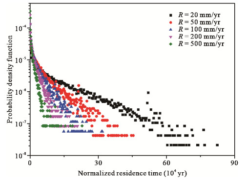
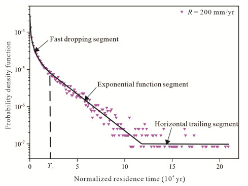
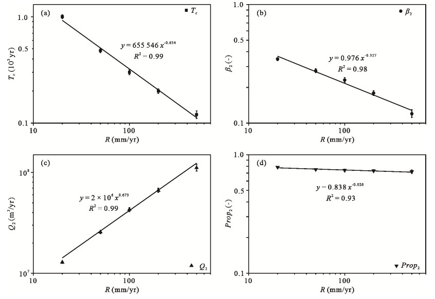
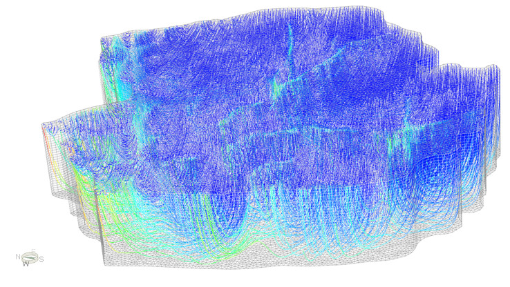
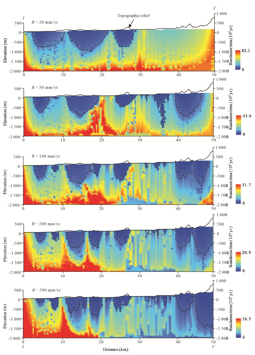
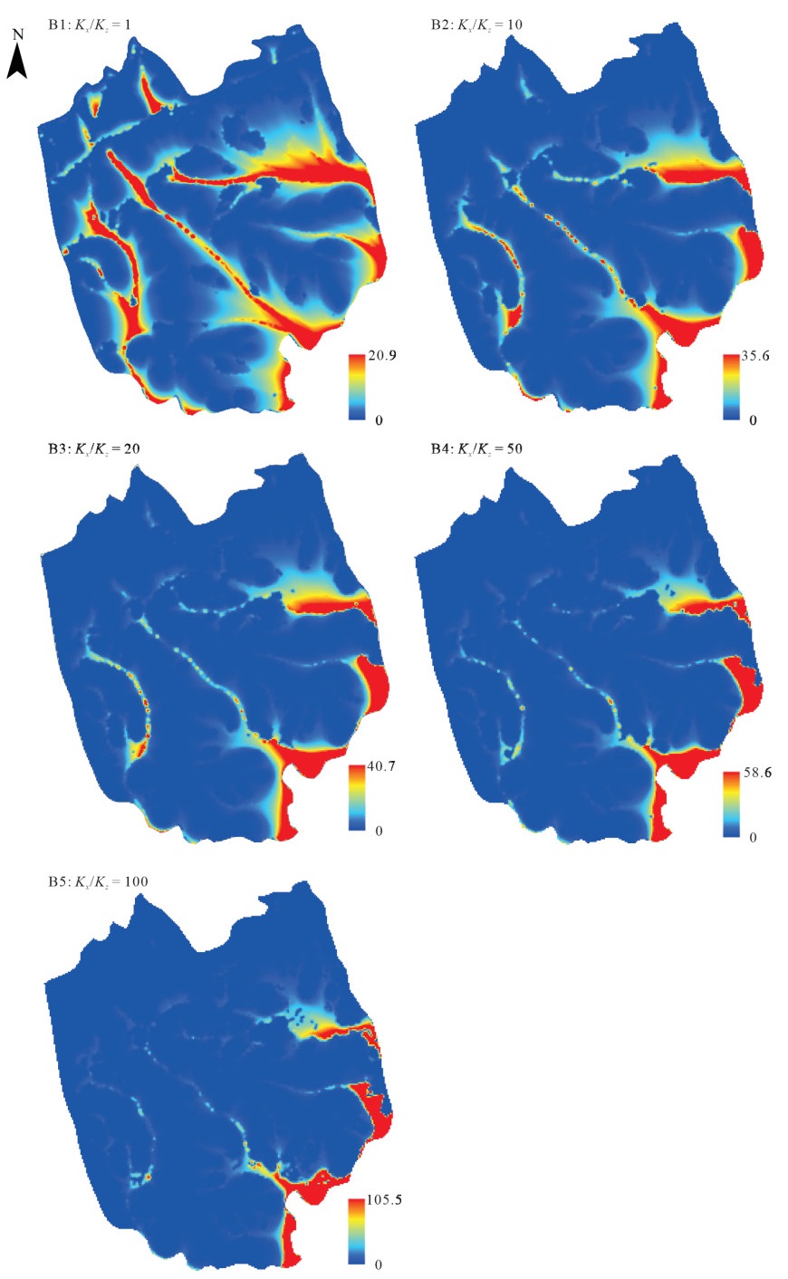
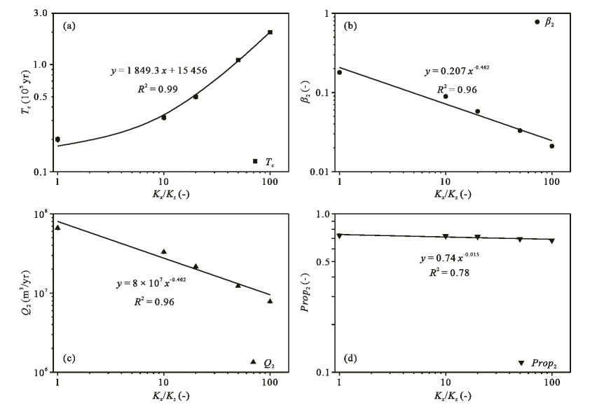
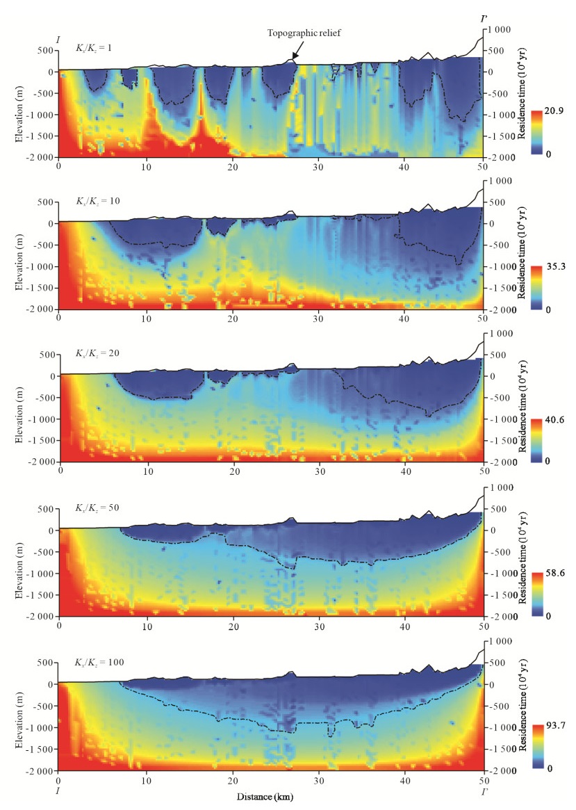
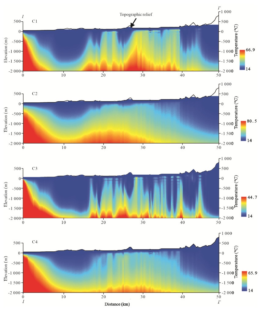
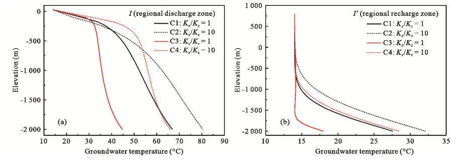
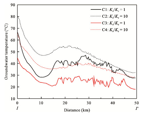
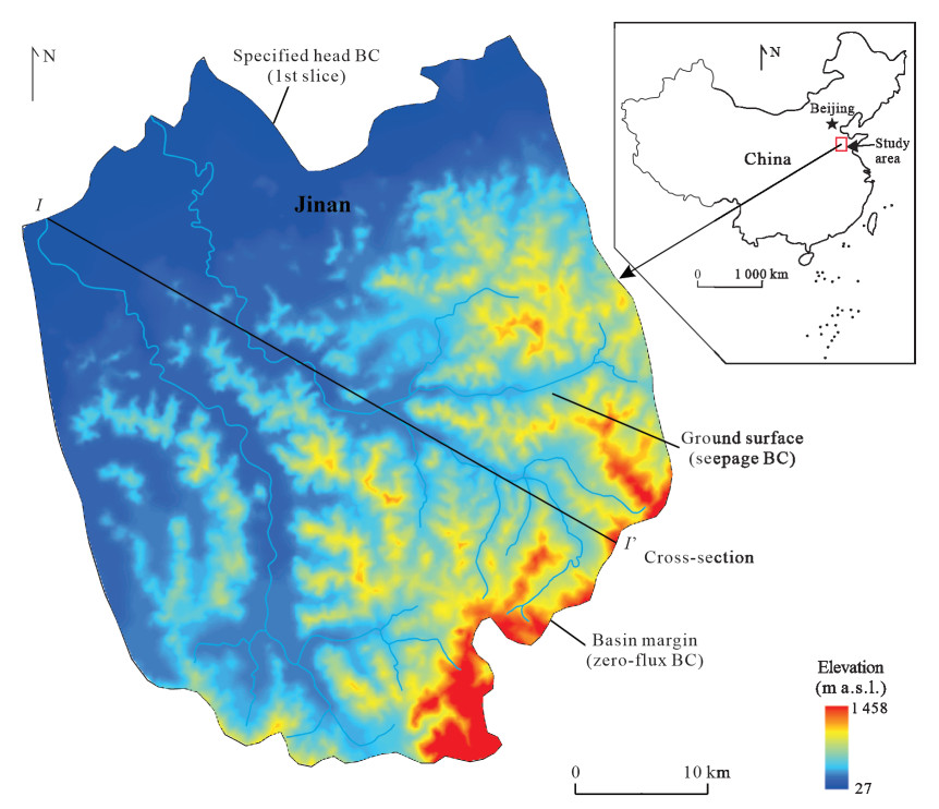
  • How to identify the nested structure of a three-dimensional (3D) hierarchical groundwater flow system is always a difficult problem puzzling hydrogeologists due to the multiple scales and complexity of the 3D flow field. The main objective of this study was to develop a quantitative method to partition the nested groundwater flow system into different hierarchies in three dimensions. A 3D numerical model with topography derived from the real geomatic data in Jinan, China was implemented to simulate groundwater flow and residence time at the regional scale while the recharge rate, anisotropic permeability and hydrothermal effect being set as climatic and hydrogeological variables in the simulations. The simulated groundwater residence time distribution showed a favorable consistency with the spatial distribution of flow fields. The probability density function of residence time with discontinuous segments indicated the discrete nature of time domain between different flow hierarchies, and it was used to partition the hierarchical flow system into shallow/intermediate/deep flow compartments. The changes in the groundwater flow system can be quantitatively depicted by the climatic and hydrogeological variables. This study provides new insights and an efficient way to analyze groundwater circulation and evolution in three dimensions from the perspective of time domain.


  • Electronic Supplementary Materials: Supplementary materials (Figs. S1–S3) are available in the online version of this article at https://doi.org/10.1007/s12583-022-1623-3.
  • The groundwater flow system theory reveals the systemic and structural properties of groundwater flow, and is a useful tool to study groundwater circulation and evolution (Tóth, 2009). At the basin scale, the pattern of groundwater circulation has been found to be organized into hierarchical sets of flow systems, i.e., local, intermediate, and regional flow systems could develop (Tóth, 1963). Each hierarchy has its specific flow pathway and hydraulic property, which would influence the interaction between groundwater and its ambient environment and subsequently determine the physical and chemical properties of groundwater (Mao et al., 2021; Gil-Márquez et al., 2020; Kirchheim et al., 2019; Wang et al., 2015; Tóth, 1999). Thus identifying the groundwater flow patterns is essential for understanding the hydrological cycle and sustainable management of groundwater resources (Li et al., 2021; Wang et al., 2021; Elaid et al., 2020; Tóth et al., 2016; Kagabu et al., 2011). This however still remains difficult especially for large areas (Cao et al., 2016; Wang J-Z et al., 2016; Goderniaux et al., 2013; Jiang et al., 2012; Yamanaka et al., 2011).

    Mathematical modeling, either analytic or numerical solutions, has been extensively used to investigate the nested groundwater flow structures and their variations with geologic and/or climatic variables (Jiang et al., 2021). The key to partition different flow hierarchies is to identify the hydraulic boundaries between them (Wang et al., 2017). Two methods are usually used. The first is to find the internal stagnation points and dividing streamlines between different flow systems (Bresciani et al., 2019; Jiang et al., 2011). The second is to analyze the spatial distribution of groundwater pathways by tracing streamlines linking recharge to discharge areas (Wang et al., 2017; Welch and Allen, 2012; Ophori, 2004). These two approaches have been found quite effective to diagnose and exhibit the nested structure of groundwater flow system in two-dimensional (2D) profiles. However, the vast majority of basin-scale groundwater flow in the real world moves in three dimensions and the complex topography can result in a more complex groundwater flow structure (Xiao et al., 2020; Kolbe et al., 2016; Marklund and Wörman, 2011; Gleeson and Manning, 2008). If groundwater flow in such cases is represented by 2D models, certain hydrological processes would be missed, which may even influence the characterization of groundwater flow system. Therefore, a thorough understanding on the actual basin-scale groundwater circulation should be based on 3D analyses.

    Due to the strict mathematical definition of stagnation points where the groundwater velocity is zero (Jiang et al., 2011; Bear, 1972), it is difficult to accurately locate the internal stagnation points in a complex 3D groundwater basin (Wang J-Z et al., 2016). Even if accurately located, it is also difficult to determine the associated dividing flow surfaces. If using the streamline tracing method, as groundwater pathways are always not legible in a complex 3D groundwater basin due to the superposition effect of different spatial scales, delineating the spatial distribution of different flow systems in three dimensions is another huge challenge (Seidel et al., 2014; Gleeson and Manning, 2008).

    Groundwater residence time, which is the total time required by water particles to move from recharge to discharge areas (Cornaton and Perrochet, 2006), contains a lot of hydrogeological information about groundwater circulation, and it can be used as a comprehensive indicator for groundwater flow and transport (Zhu et al., 2021; Land and Timmons, 2016; Lapworth et al., 2013). Groundwater in the system moves from specific recharge areas and terminates in the corresponding discharge areas with spatiotemporal orderly structures (Xu et al., 2021; Tóth, 2009). In the same hierarchy, groundwater follows the same hydraulic pattern with similar hydrodynamic behavior and their spatiotemporal attributes in different flowlines change with continuous gradient. However, groundwater from different hierarchies has distinct spatiotemporal attributes and hydraulic boundaries exist between them (Wang et al., 2017; Liang et al., 2015). For instance, the internal stagnation point used to identify different subsurface flow systems just corresponds to the location where the hydrodynamic behavior of groundwater flow mutates discontinuously.

    Given the spatiotemporal orderly organization of groundwater flow system, it is hypothesized that the discreteness in the spatial domain between different flow hierarchies would be reflected on the time domain. Goderniaux et al. (2013) proposed a methodology for partitioning a groundwater basin into shallow local and deep regional flow compartments according to the discreteness of groundwater residence time distribution. But Wang J-Z et al. (2016) demonstrated that the compartments partitioned by Goderniaux et al. (2013) were not identical to the local/intermediate/regional flow systems defined by Tóth (1963). The late-time peaks on the probability density function curves of residence time were found to be effective indicators to partition the hierarchies of groundwater flow system (Wang J-Z et al., 2016). However, the facts which should be considered when studying the groundwater circulation in the regional-scale deep basin, such as the anisotropy and hydrothermal effect (Liu et al., 2020; Moran-Ramírez et al., 2020), were not yet taken into account. Although An et al. (2015) had examined the effect of thermal convection on the groundwater temperature distribution in a 2D Tóthian basin, they assumed the hydraulic conductivity being constant and neglected the hydrothermal effect that water density and viscosity were temperature-dependent during the simulation.

    The main objective of this study was to identify the hierarchically nested structure of a 3D groundwater flow system at the basin scale. Within this context, we developed a numerical model to simulate groundwater flow and residence time. Groundwater flows were considered in three dimensions and organized across several scales from small catchment to the basin scale. The simulation results were used to examine the relationship between the residence time distribution and the hierarchically nested structure in space, attempting to partition the 3D groundwater flow system into different subsurface compartments. The model was subsequently used to investigate how the characteristics of groundwater flow system were affected by a variety of climatic and hydrogeological settings including recharge rate, anisotropic permeability and hydrothermal effect.

    A numerical model was developed to simulate groundwater flow in three dimensions for a synthetic case. Groundwater flow was assumed to be in a steady state. Since the main objective of the present study was not to represent real geological conditions but to explore a general method to identify the nested structure of a generic 3D groundwater flow system, the specific or complicated geological conditions were eliminated from the modeling. A homogeneous aquifer was assumed in the simulations.

    For convenience, the real digital elevations derived from Jinan, where the groundwater system is representative of that in northern China (Wang J L et al., 2016), were chosen to define the model topography, enabling the complexity of topographic relief to be included in the groundwater flow model (Fig. 1). The model area (1 800 km2) covered topographic changes from hilly land to a piedmont inclined plain, and further to the alluvial plain, with altitudes varying from 27 to 1 458 m. The lateral limits of the model area corresponded to the hydrogeological boundaries of Jinan groundwater system (Kang et al., 2011), and the vertical extensions ranged from ground surface to the elevation of 2 000 m below sea level.

    Figure  1.  General view of model area, topographic relief and boundary conditions (map of China after GS(2016)1555).

    In this synthetic modeling, a seepage boundary condition was prescribed to the top surface of the model domain (Fig. 1). Consequently, the top surface was generalized as a drainage system where groundwater can leave the system freely to feed rivers and streams when its hydraulic head was higher than the ground surface (Diersch, 2014). The most important advantage of this boundary condition was that the position and quantity of groundwater sources and sinks were not prescribed in advance, but calculated according to the recharge and aqueous media property.

    Groundwater outflowed as springs at the northern boundary and the average outflow elevation was 27 m. Thus a Dirichlet boundary condition with a specified head of 27 m was prescribed to the first slice of the northern boundary. A zero-flux boundary condition was prescribed to all the other lateral limits and to the bottom of the model domain.

    Precipitation recharge was uniformly imposed on the top surface of the model domain. Groundwater table and river network were not prescribed but dependent on recharge and aquifer property due to the seepage boundary asigned to the model top surface. The homogeneous hydraulic conductivity of the model was adjusted, in such a way, the simulated groundwater drainage location approximated to the current surface hydrographical network when the actual stationary recharge rate of 200 mm/yr in Jinan was used as an input to the model. This calibration led to a hydraulic conductivity of 0.1 m/d.

    The numerical simulation was performed with the finite element subsurface flow model program FEFLOW (version 6.2, DHI-WASY). The model area was discretized using triangular finite element meshes with similar sizes to ensure the calculation accuracy. Vertically, the model domain was equally divided into 30 layers, and subsequently 31 slices from the ground surface to the bottom. Each slice was composed of 11 818 nodes and 23 259 finite element meshes with sizes of approximately 500 m.

    The simulations were run under steady state and groundwater residence time was calculated using forward particle tracking. One particle which entered the groundwater system synchronously with precipitation infiltration was placed on each of the 11 818 nodes at the model top surface. These particles then migrated through aquifer system and finally left the system from discharge areas synchronously with groundwater. Therefore, the particle transit time from inlet to outlet corresponded to the groundwater residence time within the system.

    Consequently, 11 818 groundwater residence time samples can be acquired, and then probability density function was used to describe the residence time distribution from such a huge statistical sample cluster. The probability density function was approximated by statistically counting the prequency distribution of these residence time samples. Since the groundwater residence time was proportional to the effective porosity of aqueous media under advective regime, it was normalized by dividing the effective porosity (time/porosity) to eliminate the effect of media porosity.

    Recharge rate, anisotropic permeability and hydrothermal effect were set as variables to investigate their influence on groundwater residence time distribution. Three groups of numerical models, models A, B and C, with uniform geometric configuration and boundary conditions, but different simulation variables were designed to simulate groundwater flow patterns.

    Recharge rate was the simulation variable set in Model A with isotropic aqueous media and isothermal condition. To acquire distinct groundwater table configurations, it was set at an intentionally large range of 20–500 mm/yr in Model A (Table 1).

    Table  1.  Parameters designed in Model A
    Number Hydraulic conductivity,
    Kx= Ky= Kz (m/d)
    Recharge rate,
    R (mm/yr)
    A1 0.1 20
    A2 50
    A3 100
    A4 200
    A5 500
    A1, A2, A3, A4, A5 are serial numbers of different settings in Model A.
     | Show Table
    DownLoad: CSV

    Anisotropic permeability was the simulation variable set in Model B with the same recharge rate and isothermal condition. Permeability in the horizontal direction (Kx) is generally larger than that in the vertical direction (Kz) (Maasland, 1957). Stratified heterogeneity can even make the difference between Kx and Kz up to 2–3 orders of magnitude in some sedimentary basins (Deming, 2002). The anisotropic ratio of permeability (Kx/Kz) was set at a range of 1–100 in Model B (Table 2).

    Table  2.  Parameters designed in Model B
    Number Recharge rate,
    R (mm/yr)
    Permeability in the
    horizontal direction,
    Kx = Ky (m/d)
    Anisotropic ratio of
    permeability, Kx/Kz
    B1 200 0.1 1
    B2 10
    B3 20
    B4 50
    B5 100
    B1, B2, B3, B4, B5 are serial numbers of different settings in Model B.
     | Show Table
    DownLoad: CSV

    Hydrothermal effect was the simulation variable set in Model C with the same recharge rate and horizontal permeability. Heat transport was coupled into the fluid flow and two sub-groups were established for comparison, in which water density and viscosity were set constant and variable with temperature respectively (Table 3). Anisotropic permeability was also taken into account in Model C. It should be noted that the value of hydraulic conductivity (0.1 m/d) was just an initial input value in Model C3 and C4. A correction coefficient based on the water density and viscosity would be automatically assigned to the hydraulic conductivity during the simulation in condition of the temperature-dependent water density and viscosity.

    Table  3.  Parameters designed in Model C
    Number Simulation factors Recharge rate, R (mm/yr) Permeability in the horizontal direction, Kx = Ky (m/d) Anisotropic ratio of
    permeability, Kx/Kz
    C1 Constant water density and viscosity 200 0.1 1
    C2 10
    C3 Temperature-dependent water density and viscosity 1
    C4 10
    C1, C2, C3, C4 are serial numbers of different settings in Model C.
     | Show Table
    DownLoad: CSV

    The governing equations which coupled fluid flow and heat transport were numerically solved by FEFLOW (version 6.2, DHI-WASY). When considering the hydrothermal effect, the variable water density and viscosity influenced by temperature were implemented in the groundwater flow equation, in which the form of Darcy's law was extended, as formulated for example in Garven (1989) and Appold and Monteiro (2009). The regulations of water density and viscosity variation with temperature were referred to Magri et al. (2010) and Herbert et al. (1988), respectively.

    A constant temperature of 14 ℃, corresponding to the current average annual temperature in Jinan, was prescribed to the top boundary of the model domain. A heat flux was specified along the basal boundary. The lateral boundaries were assumed to be closed to heat flow. The parameters of heat transport in Model C were basin-scale averages from previous numerical studies and field explorations (Table 4).

    Table  4.  Parameters assigned to heat transport in Model C
    Parameter Value References
    Porosity 0.01 Cai et al. (2013)
    Thermal capacity of water 4.2 MJ·m-3·K-1 An et al. (2015)
    Thermal conductivity of water 0.6 J·m-1·s-1·K-1 An et al. (2015)
    Thermal conductivity of solid rock 3 J·m-1·s-1·K-1 Li et al. (2013)
    Longitudinal dispersivity 50 m One-thousandth of basin length (Jiang et al., 2012)
    Transverse dispersivity 5 m
    Basal heat flux 60 mW·m-2 Li et al. (2013)
     | Show Table
    DownLoad: CSV

    Spatial distributions of simulated groundwater residence time under different recharge rates were shown in Fig. 2. Groundwater residence time declined with the increase of recharge rates. Normalized residence time varied from 0 to 82.1 × 10⁴ yr for a recharge rate of 20 mm/yr, and decreased to a range of 0–18.7 × 10⁴ yr when the recharge rates increased to 500 mm/yr. Residence time decreasing amplitude got smaller as recharge rates increased. The maximum residence time almost fell by half when the recharge rates increased from 20 to 50 mm/yr, but only fell by 10% when the recharge rates increased from 200 to 500 mm/yr.

    Figure  2.  Spatial distributions of normalized groundwater residence time (time/porosity, unit: 104 yr) under different recharge rates. Data are plotted at the starting points of each forward tracking particle on the model top surface.

    The planar distribution of residence time (Fig. 2) provided a direct exhibition of groundwater recharge/discharge area distribution and evolution under different recharge rates. Groundwater discharge areas were mainly distributed in the northern plain and southern mountain valleys. Residence time increased from discharge areas to mountainous terrains, with the highest value in the topographic crests, where regional groundwater was sourced. Groundwater got younger and areas with relatively longer residence time shrank to the topographic highs as the input recharge increased. Most groundwater discharged at adjacent topographic lows and groundwater circulations were more local at higher recharge rates. On the contrary, the residence time distribution became more continuous and larger groundwater catchments appeared at lower recharge rates, emphasizing the recharge effect on groundwater flow delineation.

    The statistical distributions of groundwater residence time under different recharge rates were shown in Fig. 3, where probability density functions were used based on the 11 818 residence time samples calculated by the forward particle tracking from the model top surface. The distributions of residence time probability density functions under different recharge rates had similar structures. The shape of probability density functions tended to be flat and proportion of particles with long residence time increased as recharge rates decreased.

    Figure  3.  Probability density functions of normalized residence time (time/porosity) under different recharge rates. Data are plotted against the semi-logarithmic axes.

    The late-time peaks demonstrated by Wang J-Z et al. (2016) did not appear in the probability density function curves (Fig. 3), which indicated that only one flow hierarchy occurred in the groundwater basin. Basin geometry was an important factor controlling the pattern of groundwater flow system (Liang et al., 2013). The large ratio of basin length to depth (~50 : 2 in the present study) was not conducive to the development of nested hierarchical groundwater flow system.

    To further diagnose the structure of residence time statistical distribution, the probability density functions for the recharge rate of 200 mm/yr were taken out particularly for an explicit exhibition (Fig. 4). It was quite visible that the scatters of probability density functions can be divided into 3 segments, which were named in this paper as the fast dropping segment, exponential function segment and horizontal trailing segment in due order from the minimum residence time. Each segment corresponded to different groundwater flow regimes.

    Figure  4.  Probability density functions of normalized residence time for the recharge rate of 200 mm/yr. Data are plotted against the semi-logarithmic axes.

    By assuming Dupuit flow in 2D steady state, Haitjema (1995) found that the probability density functions of groundwater residence time could be expressed by an exponential model. However, the residence time probability density functions calculated in the present study cannot be completely depicted by an exponential distribution, as groundwater flow was simplified into a 2D planar flow in Haitjema's derivation, ignoring the effect of topographic relief on groundwater flow in three dimensions.

    Groundwater particles belonging to the fast dropping segment were characterized by short residence time, corresponding to small pathway distances and quick flow velocities. Groundwater movements in this compartment were mainly in the vertical directions and controlled by the local topography, hardly to meet the Dupuit's hypothesis. It can be inferred that this segment was primarily ascribed to the shallow flow compartment close to the topography.

    Groundwater particles belonging to the exponential function segment were characterized by relatively long residence time, corresponding to large pathway distances and slow flow velocities. Groundwater movements in this compartment were more regional and deeper. Goderniaux et al. (2013) defined this compartment as the "deep regional flow compartment". But considering that the the pattern of probability density functions acquired in the present study was a bit different from that in Goderniaux et al. (2013), including an extra trailing segment, we ascribed groundwater flow in this segment to the intermediate flow compartment.

    Groundwater particles belonging to the horizontal trailing segment were characterized by the longest residence time, corresponding to the basin-scale transfers. Groundwater movements in this compartment were controlled by the major topographic features, where streamlines were sourced from the topographic crests and ending at the lowest regions. Groundwater in this segment can be defined as the deep flow compartment.

    Therefore, groundwater particles can be classified into shallow/intermediate/deep flow compartments according to the flow regimes deduced by their residence time distribution. It should be noted that the shallow/intermediate/ deep flow compartments described in the present study were not identical to the local/intermediate/regional flow systems defined by Tóth (1963).

    Due to the limited number of particles in deep flow compartment with long residence time, the scatters in the horizontal trailing segment were aligned in a vertical stratified mode (Fig. 4), making it difficult to accurately determine the dividing point between the horizontal trailing and exponential function segments. Since the horizontal trailing segment can be regarded as a particular exponential distribution with a slope of zero in the semi-logarithmic coordinate system, and they were both controlled by the large scale topography, these two segments were merged and collectively referred to as the deep flow compartment in this paper.

    A critical residence time (Tc) between the fast dropping and exponential function segments can be ascertained from the distribution of probability density functions (Fig. 4). Scatters in the exponential function segment can be well fitted with a straight line in the semi-logarithmic coordinate system, and the left vertex of this line corresponded to the demarcation point of residence time. According to the above hydrogeological interpretation of these two segments, two compartments of the hierarchical flow system can be explicitly identified based on the criterion of Tc. Groundwater particles with residence time < Tc were ascribed to the shallow flow compartment, while the other particles with residence time > Tc were ascribed to the deep flow compartment.

    The distribution of residence time probability density functions provided insights into the structure of the 3D groundwater flow system. Parameters for quantitatively characterizing each flow compartment can be calculated by the following equations (Goderniaux et al., 2013)

    Qi=βi×AT×R(1) (1)
    Vi=Qi×Ti/ne=Qi×Ti(2) (2)

    where Qi [L3·T-1] was the recharge flux associated to compartment i; βi [-] was the proportion of groundwater particles attributed to compartment i; AT [L2] was the area of the model top surface; R [L·T-1] was the recharge rate; Vi [L3] was the saturated aquifer volume associated to compartment i; Ti [T] was the average residence time associated to compartment i; ne [-] was the effective porosity of the aqueous media; Ti* [T] was the average normalized residence time associated to compartment i; i = 1 corresponded to the shallow flow compartment and i = 2 corresponded to the deep flow compartment.

    Due to the discrete nature of the residence time sample cluster, a deviation would occur when determining the demarcation point of residence time. This deviation was sourced from the class interval during the statistical calculation of probability density function, which constituted the upper/lower limit of error margin for the parameter Tc. The ranges of other parameters β2, Q2 and Prop2 can be calculated accordingly.

    As shown in Table 5, with the recharge rates decreasing from 500 to 20 mm/yr, the critical residence time (Tc) increased from 12 000 to 100 000 yr, indicating a constrained groundwater penetration ability and declined movement velocities. With lower recharge rates, the relative (β2) and absolute (Q2) deep flow flux increased and decreased, respectively, while the volume proportion of deep flow compartment to the total saturated aquifer (Prop2) increased slightly.

    Table  5.  Parameters for characterizing groundwater flow system under different recharge rates
    R (mm/yr) Tc (×104 yr) β2 (-) Q2 (×107 m3/yr) T2*(×104 yr) V2 (×1012 m3) Prop2 (-)
    20 10 (-0.40, +0.40) 0.35 (-0.01, +0.01) 1.29 (-0.04, +0.04) 23.83 (-0.39, +0.41) 3.07 (-0.04, +0.04) 0.78 (-0.01, +0.01)
    50 4.8 (-0.20, +0.20) 0.28 (-0.01, +0.01) 2.56 (-0.09, +0.11) 11.61 (-0.27, +0.24) 2.97 (-0.04, +0.05) 0.75 (-0.01, +0.01)
    100 3 (-0.15, +0.15) 0.23 (-0.01, +0.01) 4.28 (-0.19, +0.21) 6.88 (-0.18, +0.18) 2.95 (-0.06, +0.06) 0.74 (-0.01, +0.02)
    200 2 (-0.10, +0.10) 0.18 (-0.01, +0.01) 6.64 (-0.30, +0.34) 4.42 (-0.12, +0.11) 2.94 (-0.06, +0.07) 0.73 (-0.02, +0.02)
    500 1.2 (-0.10, +0.10) 0.12 (-0.01, +0.01) 11.13 (-0.79, +0.93) 2.62 (-0.11, +0.10) 2.92 (-0.10, +0.11) 0.72 (-0.02, +0.03)
    R. Recharge rate; Tc. critical residence time; β2. proportion of deep flow particles; Q2. recharge flux of deep flow; T2*. the average normalized residence time of deep flow compartment; V2. the saturated aquifer volume of deep flow compartment; Prop2. volume proportion of deep flow. The negative/ positive value in the brackets represents the lower/upper limit of error margin for each parameter, respectively.
     | Show Table
    DownLoad: CSV

    As shown in Fig. 5, the changes in parameter Tc, β2, Q2 and Prop2 with recharge rate were all best fitted by power laws, providing a quantitative characterization of groundwater flow system response to recharge variation. Although the mechanism of the above functions was not yet clear and may need to be further studied by analytical method, it enabled the critical residence time, recharge flux and volume of shallow/deep flow compartment to be quickly estimated in a convenient way.

    Figure  5.  Diagrams showing the changes in (a) the critical residence time Tc, (b) proportion of deep flow particles β2, (c) recharge flux of deep flow Q2, (d) volume proportion of deep flow Prop2 as a function of the recharge rate. The error bar indicates the upper and lower limits of error margin for each parameter.

    As shown in Table 5 and Fig. 5, the deviations of other characteristic parameters were relatively small, indicating that although Tc was not strictly accurate to a specific value, the deviation could only marginally affect the division of the groundwater flow systems.

    As it was difficult to achieve the visualization of nested flow patterns in three dimensions which were really complicated and dizzying (Fig. 6, taking the simulation result of Model A4 as an example), a profile (I-I' section in Fig. 1) was used to demonstrate the flow system partitioning intuitively. Figure 7 presents the residence time distribution of groundwater particles across the profile. According to the definition of residence time, groundwater particles belonging to the same streamline had equal residence time, so the isolines/isosurfaces of residence time corresponded to the groundwater flow lines/planes. Therefore the residence time distribution across the profile presents a visual revelation of the groundwater flow patterns. Since most of the groundwater flow lines, including horizontal and vertical flows, were orthogonal or oblique to the profile, rather than completely flowing along the profile, some abrupt changes in residence time occurred on the profile and presented like noise points, but it would not affect the overall interpretation of the flow system.

    Figure  6.  The complicated 3D groundwater flow fields simulated in Model A4 (vertical exaggeration: 5×). The streamline color changing from blue to green to red indicated groundwater age became older along the direction of groundwater flow.

    As shown in Fig. 7, groundwater penetration ability became constrained and water movement tended to be horizontal and succinct with lower recharge rate. On the contrary, with the increase of recharge rate, the residence time decreased and groundwater flow pattern tended to be complex. When the recharge rate exceeded 100 mm/yr, groundwater residence time in the southern mountainous area presented an indented distribution. With higher recharge rates, groundwater penetration ability became powered and facilitated shallow flow compartment developing to the depth, which was especially obvious in the southern mountainous area with larger gravitational potential. Meanwhile more and more sub-catchments were partitioned from the shallow compartment, indicating the incision of topographic relief became increasingly evident.

    Figure  7.  Normalized groundwater residence time distribution across the profile I-I' under different recharge rates. The dotted line as the isoline of Tc in the profile is the interface between shallow and deep flow compartments. The I-I' section is labelled in Fig. 1.

    As shown in Fig. 8, groundwater residence time increased with the anisotropic ratio of permeability (Kx/Kz). Low vertical hydraulic conductivity (Kz) resulted in a poor groundwater penetration ability, leading to the discharge area with short residence time expanding, while the recharge area where regional groundwater was sourced shrinking to the topographic highs.

    Figure  8.  Spatial distributions of normalized groundwater residence time (time/porosity, unit: 104 yr) with different anisotropic ratio of permeability (Kx/Kz). Data are plotted at the starting points of each forward tracking particle on the model top surface.

    With the increase of Kx/Kz, the distribution of residence time probability density functions gradually transited from three-segment type (fast dropping, exponential function and horizontal trailing segments) to two-segment type (fast dropping and horizontal trailing segments), in which the exponential function segment corresponding to the intermediate flow compartment gradually contracted until disappeared (Fig. 9). This transition indicates that with the increase of Kx/Kz, groundwater flow pattern gradually changed from the shallow-intermediate-deep nested system to the simple shallow-deep nested system.

    Figure  9.  Diagrams showing the probability density functions of normalized residence time with different anisotropic ratio of permeability (Kx/Kz). Data are plotted against the semi-logarithmic axes.

    Parameters for quantitatively characterizing the groundwater flow system simulated in Model B were calculated by Eqs. (1), (2) and summarized in Table 6. As Kx/Kz increased from 1 to 100, the critical residence time (Tc) increased from 20 000 to 200 000 yr, the relative deep flow flux (β2) decreased from 0.18 to 0.02, and the recharge flux of deep compartment (Q2) decreased significantly from 6.64 × 10⁷ to 0.78 × 10⁷ m3/yr, indicating that the deep regional groundwater flow was gradually turned into local flow with shallow and short circulation. Prop2 varied in a limited range of 0.68–0.73, indicating that Kx/Kz could only marginally modify the volume proportion attributed to the deep/shallow flow compartment.

    Table  6.  Parameters for characterizing groundwater flow system with different anisotropic ratio of permeability (Kx/Kz)
    Kx/Kz (-) Tc (×104 yr) β2 (-) Q2 (×107 m3/yr) T2*(×104 yr) V2 (×1012 m3) Prop2 (-)
    1 2 (-0.10, +0.10) 0.18 (-0.01, +0.01) 6.64 (-0.30, +0.34) 4.42 (-0.12, +0.11) 2.94 (-0.06, +0.07) 0.73 (-0.02, +0.02)
    10 3.2 (-0.15, +0.15) 0.09 (-0.003, +0.004) 3.30 (-0.12, +0.13) 8.89 (-0.22, +0.22) 2.93 (-0.04, +0.04) 0.72 (-0.01, +0.01)
    20 5 (-0.20, +0.20) 0.06 (-0.002, +0.002) 2.15 (-0.08, +0.06) 13.58 (-0.22, +0.32) 2.92 (-0.04, +0.03) 0.72 (-0.01, +0.01)
    50 11 (-0.25, +0.25) 0.03 (-0.000 3, +0.000 3) 1.22 (-0.01, +0.01) 23.20 (-0.12, +0.12) 2.84 (-0.01, +0.01) 0.70 (-0.003, +0.003)
    100 20 (-0.50, +0.50) 0.02 (-0.000 7, +0.000 6) 0.78 (-0.03, +0.02) 35.82 (-0.44, +0.52) 2.79 (-0.05, +0.04) 0.68 (-0.01, +0.01)
    Kx/Kz. Anisotropic ratio of permeability; Tc. critical residence time; β2. proportion of deep flow particles; Q2. recharge flux of deep flow; T2*. the average normalized residence time of deep flow compartment; V2. the saturated aquifer volume of deep flow compartment; Prop2. volume proportion of deep flow. The negative/positive value in the brackets represents the lower/upper limit of error margin for each parameter, respectively.
     | Show Table
    DownLoad: CSV

    As shown in Fig. 10, a favorable linear relationship between Tc and Kx/Kz was obtained, while the changes in parameter β2, Q2 and Prop2 with Kx/Kz were best fitted by power laws. These empirical functions provided a quantitative characterization of groundwater flow system response to the variation of Kx/Kz, and also offered a convenient way to quickly estimate the characteristic parameters of groundwater flow system, although the inherent mechanism was not clear at present.

    Figure  10.  Diagrams showing the changes in the (a) critical residence time Tc, (b) proportion of deep flow particles β2, (c) recharge flux of deep flow Q2, (d) volume proportion of deep flow Prop2 as a function of the anisotropic ratio of permeability (Kx/Kz). The error bar, indicating the upper and lower limits of error margin for each parameter, is very small and hard to be distinguished in the figure.

    Figure 11 exhibits the residence time distribution of groundwater particles across the profile I-I', and gave a direct visualization of groundwater flow patterns with different Kx/Kz. With the increase of Kx/Kz, groundwater penetration depth decreased and water movement tended to be horizontal, making groundwater flow patterns appear to be more compendious. Meanwhile sub-catchments in shallow flow compartment dissected by the topography were gradually merged into a large scale compartment with longer flow distances, indicating the restriction of anisotropic aqueous media on the spatial development of groundwater flow system.

    Figure  11.  Normalized groundwater residence time distribution across the profile I-I' with different anisotropic ratio of permeability (Kx/Kz). The dotted line as the isoline of Tc in the profile is the interface between shallow and deep flow compartments. The I-I' section is labelled in Fig. 1.

    Taking the profile I-I' for instance, the distributions of groundwater temperature across the profile simulated in Model C are illustrated in Fig. 12. Below the constant temperature zone, groundwater temperature increased with depth and reached the highest at the bottom below the regional discharge zone. The descending groundwater flow below recharge area received the cooling infiltration water, driving the isotherms to move downward with larger intervals and geothermal gradient to decrease, while the ascending groundwater flow below discharge area was heated by the deep terrestrial heat flux, causing the isotherms to move upward with smaller intervals and geothermal gradient to become larger.

    Figure  12.  Distributions of groundwater temperature across the profile I-I' simulated in Model C.

    As shown in Fig. 12, groundwater temperature increased significantly with the increase of Kx/Kz. The effect of Kx/Kz on groundwater flow was also demonstrated by the temperature field. With the increase of Kx/Kz, groundwater penetration ability was constrained and water movement tended to be horizontal. The corresponding variation reflected on the groundwater temperature field was that the vertical staggered isotherms tended to spread out in the horizontal direction.

    The vertical temperature profiles in the regional discharge zone (through the northern vertex I) and in the regional recharge zone (through the southern endpoint I') are shown in Fig. 13. Groundwater temperature increased nonlinearly with depth and reached the highest at the basin bottom. The curve for the discharge zone exhibits a convex trend, while that for the recharge zone had a concave trend, indicating the difference of geothermal gradient between these two zones. The maximum temperature at the basin bottom decreased with decreasing anisotropic ratio (Kx/Kz). As Kx/Kz decreased, Kz increased when Kx was set as a constant, leading to the increase of vertical flow. More cooling water brought by the stronger vertical convective flow produced a decreasing maximum temperature in the basin.

    Figure  13.  The vertical temperature profiles through the northern vertex I (a) and southern endpoint I' (b) of the I-I' section.

    As shown in Figs. 12 and 13, when considering the hydrothermal effect that water density and viscosity was temperature-dependent, the maximum groundwater temperature was much lower than that simulated in models C1 and C2, and the maximum decrease was about 20 ℃. In models C3 and C4, water viscosity decreased with temperature, leading to the increase of hydraulic conductivity, which further promoted the convective degree in the basin. The high degree of flow and heat convection led to the decrease of vertical temperature variance as well as the geothermal gradient in the basin.

    Another difference when considering the hydrothermal effect was that groundwater temperature in the shallow depth of regional discharge zone was higher than that simulated in models C1 and C2, which was more obvious in the anisotropic condition (Fig. 13a). In models C3 and C4, as water density decreased with temperature, the low-density groundwater was subjected to the upward buoyancy, which accelerated the heat transport with upward flow to the regional discharge zone.

    The horizontal temperature profile at the basin bottom along the I-I' section was shown in Fig. 14. From the right to the left in the figure, i.e., from the recharge to the discharge zone, groundwater temperature exhibited an ascending trend with some ups and downs. Due to the topographic relief, the convergency and divergency of groundwater flow produced the ridge of local high temperature anomaly and the valley of local low temperature anomaly, respectively. Higher anisotropic ratio (Kx/Kz), corresponding to the the smaller Kz when Kx being set as a constant, smoothed the temperature undulation at the basin bottom due to the relatively low degree of vertical convection. When considering the hydrothermal effect, due to the larger hydraulic conductivity with increasing temperature, groundwater temperature at the basin bottom exhibited an overall decline with smaller fluctuation amplitude, compared to the results simulated in models C1 and C2.

    Figure  14.  Groundwater temperature distribution at the basin bottom along the I-I' section.

    As shown in Fig. S1, the spatial distribution of groundwater residence time significantly varied when considering the hydrothermal effect. Residence time as well as the extension of recharge areas where regional groundwater was sourced dramatically decreased in condition of the temperature-dependent water density and viscosity. Areas with relatively long residence time were transferred to the northern plain, which was especially obvious when comparing the results of models C1 and C3 in condition of the isotropic aqueous media.

    The distributions of residence time probability density functions with different scenarios of whether or not water density and viscosity being variable with temperature were compared in Fig. S2. The function scatters were shifted to the direction of short residence time when considering the hydrothermal effect, indicating that the proportion of groundwater particles with short residence time became larger. The exponential function segment in Model C3 was contracted in comparison with the result of Model C1, and even disappeared in the result of Model C4 with anisotropic aqueous media. This indicates that the hydrothermal effect would induce the groundwater flow pattern to convert from the shallow-intermediate-deep nested system to the shallow-deep nested system, in which intermediate compartment was gradually transferred into the shallow flow compartment.

    Parameters for quantitatively characterizing the groundwater flow system simulated in Model C were summarized in Table 7. Since water density was variable with temperature when considering the hydrothermal effect, leading to the difficulty in calculating groundwater volume, the volume and its proportion of different groundwater flow compartment were not calculated in this section. The critical residence time (Tc), as well as the relative (β2) and absolute (Q2) values of deep flow flux all decreased significantly when considering the hydrothermal effect. The influence of the anisotropic ratio of permeability (Kx/Kz) on the characteristic parameters when considering the hydrothermal effect was consistent with the results of Model B.

    Table  7.  Parameters for characterizing groundwater flow system when considering the hydrothermal effect
    Simulation factors Kx/Kz (-) Tc (×104 yr) β2 (-) Q2 (×107 m3/yr)
    Constant water density and viscosity 1 2 (-0.10, +0.10) 0.18 (-0.01, +0.01) 6.64 (-0.30, +0.34)
    10 3.2 (-0.15, +0.15) 0.09 (-0.003, +0.004) 3.30 (-0.12, +0.13)
    Temperature-dependent water density and viscosity 1 0.68 (-0.04, +0.04) 0.04 (-0.002, +0.002) 1.54 (-0.07, +0.09)
    10 2.5 (-0.07, +0.07) 0.02 (-0.000 5, +0.000 3) 0.71 (-0.02, +0.01)
    Kx/Kz. Anisotropic ratio of permeability; Tc. critical residence time; β2. proportion of deep flow particles; Q2. recharge flux of deep flow. The negative/positive value in the brackets represents the lower/upper limit of error margin for each parameter, respectively.
     | Show Table
    DownLoad: CSV

    Figure S3 exhibits the hydrothermal effect on the residence time distribution of groundwater particles across the profile I-I'. Residence time significantly decreased and shallow flow compartment was developing to the depth when considering the hydrothermal effect. Below the constant temperature zone, groundwater was heated by the deep terrestrial heat flux and water viscosity decreased in turn. The lower water viscosity resulted in a higher hydraulic conductivity and more powered penetration ability, driving more fresh water to move to the depth. On the other hand, water density also decreased with the increase of temperature, and the low-density groundwater was subjected to the upward buoyancy, which would accelerate the groundwater upward moving and make residence time below discharge area become shorter when comparing to the constant water density and viscosity condition.

    According to the simulated distributions of groundwater temperature and residence time (Figs. 12, S3), it can be seen that groundwater movement and temperature influenced each other and were mutually causal: temperature affected groundwater movement by changing water viscosity and density, while groundwater movement affected temperature distribution by fluid convection. Therefore, the groundwater temperature affected by the fluid convection was a natural tracer to indicate groundwater movement.

    Groundwater flow was gravity driven and controlled by the topography and/or recharge when the hydrothermal effect was not taken into account (Liang et al., 2013; Haitjema and Mitchell-Bruker, 2005; Tóth, 1963). But if there existed a basal heat source continuously transferring heat flux upward and its influence on groundwater flow increased to a certain extent, this stress source with high temperature cannot be ignored. Fluid particles would get mixed with each other and their tracks became quite irregular. Groundwater flow would deviate from the pattern delineated just according to the gravitational system (Tóth et al., 2020; Magri et al., 2010), making it more difficult to quantitatively depict groundwater flow system.

    A regional-scale groundwater flow numerical model was developed to study the characterization of residence time distribution in the 3D groundwater basin. The simulated groundwater residence time distribution showed a favorable consistency with the spatial distribution of flow fields. Probability density function was used to quantitatively describe the groundwater residence time statistical distribution. Each segment in the function distribution was associated to the specific groundwater flow hierarchy. A critical residence time (Tc) can be recognized from the discrete feature of residence time distribution, and it was used to partition the hierarchical groundwater flow system into shallow and deep flow compartments.

    Recharge rate, anisotropic permeability and hydrothermal effect were set as variables to investigate their influence on groundwater residence time distribution. A series of characteristic parameters was acquired to quantitatively indicate the changes in the groundwater flow system under the impact of those climatic and hydrogeological factors. The results were summarized as follows.

    (1) With the increase of recharge rate, shallow flow compartment was developing to the depth, and more sub-catchments were partitioned from the shallow compartment. The incision of topographic relief on the shallow flow compartment became increasingly evident. The proportion of the total recharge feeding the deep compartment (β2) decreased as recharge increased (∝R-0.327), while the absolute recharge flux to this compartment (Q2) increased with the total recharge (∝R0.673). The critical residence time (Tc) decreased as recharge increased (∝R-0.654). The volume proportion of deep flow compartment to the total saturated aquifer (Prop2) decreased slightly when recharge increased (∝R-0.026).

    (2) With higher anisotropic ratio of permeability (Kx/Kz), groundwater movement tended to be horizontal, and sub-catchments in shallow flow compartment dissected by the topography were gradually merged into a large scale compartment with longer flow distances. The relative (β2) and absolute (Q2) values of deep flow flux both decreased as Kx/Kz increased (∝(Kx/Kz)-0.462). The critical residence time (Tc) linearly increased with Kx/Kz. The volume proportion attributed to the deep flow compartment (Prop2) was just marginally modified by Kx/Kz (∝(Kx/Kz)-0.015).

    (3) When considering the hydrothermal effect that water density and viscosity was temperature-dependent, groundwater residence time significantly decreased and shallow flow compartment was developing to the depth. Groundwater below the regional discharge area was subjected to the upward buoyancy and its residence time became shorter when comparing to the constant water density and viscosity condition. The critical residence time (Tc), as well as the relative (β2) and absolute (Q2) values of deep flow flux all decreased significantly when considering the hydrothermal effect.

    The residence time distribution described by the probability density function was shown to be a useful tool to identify the nested structure of groundwater flow system. The modeling in this paper cannot be considered as a real regional study for the simplified and synthetic geological assumption in the simulation. But it can be regarded as an exploration hoping to provide direction for the identification of groundwater flow pattern in three dimensions.

    Future work will take into consideration the effect of geological structure and human activity on the modeling. It can be speculated that several more critical dividing points may appear in the residence time distribution when the complex geological conditions such as heterogeneity of karst development, faults with different hydraulic properties, etc. are imposed. The artificial exploitation of groundwater may also affect the residence time distribution. Therefore, the hydrogeological connotation involved in the residence time distribution should be firstly distinguished when using it for characterizing groundwater flow system.

    ACKNOWLEDGMENTS: This study was supported by the National Natural Science Foundation of China (Nos. 41807219, 41877192, U1906209, 42072331), the National Key R & D Program of China (No. 2017YFC0505304), and the Fundamental Research Funds for Central Public Welfare Research Institutes (Nos. CKSF 2019170/TB, CKSF 2016029/TB). Special thanks to the two anonymous reviewers who helped us significantly enhance the quality of this manuscript. The authors are also grateful to Dr. Jun-Zhi Wang, Yellow River Engineering Consulting Co., Ltd., for the constructive suggestions on the manuscript revision. The final publication is available at Springer via https://doi.org/10.1007/s12583-022-1623-3.
  • An, R., Jiang, X. -W., Wang, J. -Z., et al., 2015. A Theoretical Analysis of Basin-Scale Groundwater Temperature Distribution. Hydrogeology Journal, 23(2): 397–404. https://doi.org/10.1007/s10040-014-1197-y
    Appold, M. S., Monteiro, L. V. S., 2009. Numerical Modeling of Hydrothermal Zinc Silicate and Sulfide Mineralization in the Vazante Deposit, Brazil. Geofluids, 9(2): 96–115. https://doi.org/10.1111/j.1468-8123.2009.00245.x
    Bear, J., 1972. Dynamics of Fluids in Porous Media. Elsevier, New York
    Bresciani, E., Kang, P. K., Lee, S., 2019. Theoretical Analysis of Groundwater Flow Patterns near Stagnation Points. Water Resources Research, 55(2): 1624–1650. https://doi.org/10.1029/2018wr023508
    Cai, W., Gao, Z., Wang, Q., et al., 2013. Research on Connections between Jinan Karst Waters. Geological Publishing House, Beijing (in Chinese)
    Cao, G. L., Han, D. M., Currell, M., et al., 2016. Revised Conceptualization of the North China Basin Groundwater Flow System: Groundwater Age, Heat and Flow Simulations. Journal of Asian Earth Sciences, 127: 119–136. https://doi.org/10.1016/j.jseaes.2016.05.025
    Cornaton, F., Perrochet, P., 2006. Groundwater Age, Life Expectancy and Transit Time Distributions in Advective-Dispersive Systems: 1. Generalized Reservoir Theory. Advances in Water Resources, 29(9): 1267–1291. https://doi.org/10.1016/j.advwatres.2005.10.009
    Deming, D., 2002. Introduction to Hydrogeology. McGraw-Hill, New York
    Diersch, H. J. G., 2014. FEFLOW—Finite Element Modeling of Flow, Mass and Heat Transport in Porous and Fractured Media. Springer-Verlag, Berlin, Heidelberg
    Elaid, M., Hind, M., Abdelmadiid, B., et al., 2020. Contribution of Hydrogeochemical and Isotopic Tools to the Management of Upper and Middle Cheliff Aquifers. Journal of Earth Science, 31(5): 993–1006. https://doi.org/10.1007/s12583-020-1293-y
    Garven, G., 1989. A Hydrogeologic Model for the Formation of the Giant Oil Sands Deposits of the Western Canada Sedimentary Basin. American Journal of Science, 289(2): 105–166. https://doi.org/10.2475/ajs.289.2.105
    Gil-Márquez, J. M., De la Torre, B., Mudarra, M., et al., 2020. Complementary Use of Dating and Hydrochemical Tools to Assess Mixing Processes Involving Centenarian Groundwater in a Geologically Complex Alpine Karst Aquifer. Hydrological Processes, 34(20): 3981–3999. https://doi.org/10.1002/hyp.13848
    Gleeson, T., Manning, A. H., 2008. Regional Groundwater Flow in Mountainous Terrain: Three-Dimensional Simulations of Topographic and Hydrogeologic Controls. Water Resources Research, 44(10): W10403. https://doi.org/10.1029/2008wr006848
    Goderniaux, P., Davy, P., Bresciani, E., et al., 2013. Partitioning a Regional Groundwater Flow System into Shallow Local and Deep Regional Flow Compartments. Water Resources Research, 49(4): 2274–2286. https://doi.org/10.1002/wrcr.20186
    Haitjema, H. M., 1995. On the Residence Time Distribution in Idealized Groundwatersheds. Journal of Hydrology, 172(1): 127–146. https://doi.org/10.1016/0022-1694(95)02732-5
    Haitjema, H. M., Mitchell-Bruker, S., 2005. Are Water Tables a Subdued Replica of the Topography? Ground Water, 43(6): 781–786. https://doi.org/10.1111/j.1745-6584.2005.00090.x
    Herbert, A. W., Jackson, C. P., Lever, D. A., 1988. Coupled Groundwater Flow and Solute Transport with Fluid Density Strongly Dependent Upon Concentration. Water Resources Research, 24(10): 1781–1795. https://doi.org/10.1029/wr024i010p01781
    Jiang, X. -W., Wang, X. -S., Wan, L., et al., 2011. An Analytical Study on Stagnation Points in Nested Flow Systems in Basins with Depth-Decaying Hydraulic Conductivity. Water Resources Research, 47(1): W01512. https://doi.org/10.1029/2010wr009346
    Jiang, X. -W., Wan, L., Ge, S. M., et al., 2012. A Quantitative Study on Accumulation of Age Mass around Stagnation Points in Nested Flow Systems. Water Resources Research, 48(12): W12502. https://doi.org/10.1029/2012wr012509
    Jiang, L. Q., Sun, R., Liang, X., 2021. Predicting Groundwater Flow and Solute Transport in the Heterogeneous Aquifer Sandbox Using Different Parameter Estimation Methods. Earth Science, 46(11): 4150–4160. https://doi.org/10.3799/dqkx.2020.268 (in Chinese with English Abstract)
    Kagabu, M., Shimada, J., Delinom, R., et al., 2011. Groundwater Flow System under a Rapidly Urbanizing Coastal City as Determined by Hydrogeochemistry. Journal of Asian Earth Sciences, 40(1): 226–239. https://doi.org/10.1016/j.jseaes.2010.07.012
    Kang, F. X., Jin, M. G., Qin, P. R., 2011. Sustainable Yield of a Karst Aquifer System: A Case Study of Jinan Springs in Northern China. Hydrogeology Journal, 19(4): 851–863. https://doi.org/10.1007/s10040-011-0725-2
    Kirchheim, R. E., Gastmans, D., Chang, H. K., et al., 2019. The Use of Isotopes in Evolving Groundwater Circulation Models of Regional Continental Aquifers: The Case of the Guarani Aquifer System. Hydrological Processes, 33(17): 2266–2278. https://doi.org/10.1002/hyp.13476
    Kolbe, T., Marçais, J., Thomas, Z., et al., 2016. Coupling 3D Groundwater Modeling with CFC-Based Age Dating to Classify Local Groundwater Circulation in an Unconfined Crystalline Aquifer. Journal of Hydrology, 543: 31–46. https://doi.org/10.1016/j.jhydrol.2016.05.020
    Land, L., Timmons, S., 2016. Evaluation of Groundwater Residence Time in a High Mountain Aquifer System (Sacramento Mountains, USA): Insights Gained from Use of Multiple Environmental Tracers. Hydrogeology Journal, 24(4): 787–804. https://doi.org/10.1007/s10040-016-1400-4
    Lapworth, D. J., MacDonald, A. M., Tijani, M. N., et al., 2013. Residence Times of Shallow Groundwater in West Africa: Implications for Hydrogeology and Resilience to Future Changes in Climate. Hydrogeology Journal, 21(3): 673–686. https://doi.org/10.1007/s10040-012-0925-4
    Li, Z., Kang, F., Liu, G., et al., 2013. Jinan Geothermal and Hot Springs. Geological Publishing House, Beijing (in Chinese)
    Li, Y., Wang, J. L., Jin, M. G., et al., 2021. Hydrodynamic Characteristics of Jinan Karst Spring System Identified by Hydrologic Time-Series Data. Earth Science, 46(7): 2583–2593. https://doi.org/10.3799/dqkx.2020.236 (in Chinese with English Abstract)
    Liang, X., Quan, D. J., Jin, M., et al., 2013. Numerical Simulation of Groundwater Flow Patterns Using Flux as Upper Boundary. Hydro-logical Processes, 27(24): 3475–3483. https://doi.org/10.1002/hyp.9477
    Liang, X., Zhang, R., Jin, M. G., 2015. Groundwater Flow Systems: Theory, Application and Investigation. Geological Publishing House, Beijing (in Chinese)
    Liu, Y. J., Ma, T., Chen, J., et al., 2020. Compaction Simulator: A Novel Device for Pressure Experiments of Subsurface Sediments. Journal of Earth Science, 31(5): 1045–1050. https://doi.org/10.1007/s12583-020-1334-6
    Maasland, M., 1957. Theory of Fluid Flow through Anisotropic Media. In: Luthin, J. N., ed., Drainage of Agricultural Lands. American Society of Agronomy, Wisconsin Madison
    Magri, F., Akar, T., Gemici, U., et al., 2010. Deep Geothermal Groundwater Flow in the Seferihisar-Balçova Area, Turkey: Results from Transient Numerical Simulations of Coupled Fluid Flow and Heat Transport Processes. Geofluids, 10(3): 388–405. https://doi.org/10.1111/j.1468-8123.2009.00267.x
    Mao, X. M., Zhu, D. B., Ndikubwimana, I., et al., 2021. The Mechanism of High-Salinity Thermal Groundwater in Xinzhou Geothermal Field, South China: Insight from Water Chemistry and Stable Isotopes. Journal of Hydrology, 593: 125889. https://doi.org/10.1016/j.jhydrol.2020.125889
    Marklund, L., Wörman, A., 2011. The Use of Spectral Analysis-Based Exact Solutions to Characterize Topography-Controlled Groundwater Flow. Hydrogeology Journal, 19(8): 1531–1543. https://doi.org/10.1007/s10040-011-0768-4
    Moran-Ramírez, J., Morales-Arredondo, J. I., Armienta-Hernández, M. A., et al., 2020. Quantification of the Mixture of Hydrothermal and Fresh Water in Tectonic Valleys. Journal of Earth Science, 31(5): 1007–1015. https://doi.org/10.1007/s12583-020-1294-x
    Ophori, D. U., 2004. A Simulation of Large-Scale Groundwater Flow and Travel Time in a Fractured Rock Environment for Waste Disposal Purposes. Hydrological Processes, 18(9): 1579–1593. https://doi.org/10.1002/hyp.1407
    Seidel, T., König, C., Schäfer, M., et al., 2014. Intuitive Visualization of Transient Groundwater Flow. Computers & Geosciences, 67: 173–179. https://doi.org/10.1016/j.cageo.2014.03.004
    Tóth, Á., Havril, T., Simon, S., et al., 2016. Groundwater Flow Pattern and Related Environmental Phenomena in Complex Geologic Setting Based on Integrated Model Construction. Journal of Hydrology, 539: 330–344. https://doi.org/10.1016/j.jhydrol.2016.05.038
    Tóth, Á., Galsa, A., Mádl-Szőnyi, J., 2020. Significance of Basin Asymmetry and Regional Groundwater Flow Conditions in Preliminary Geothermal Potential Assessment—Implications on Extensional Geothermal Plays. Global and Planetary Change, 195: 103344. https://doi.org/10.1016/j.gloplacha.2020.103344
    Tóth, J., 1963. A Theoretical Analysis of Groundwater Flow in Small Drainage Basins. Journal of Geophysical Research, 68(16): 4795–4812. https://doi.org/10.1029/jz068i016p04795
    Tóth, J., 1999. Groundwater as a Geologic Agent: An Overview of the Causes, Processes, and Manifestations. Hydrogeology Journal, 7(1): 1–14. https://doi.org/10.1007/s100400050176
    Tóth, J., 2009. Gravitational Systems of Groundwater Flow. Cambridge University Press, New York
    Wang, J. -Z., Wörman, A., Bresciani, E., et al., 2016. On the Use of Late-Time Peaks of Residence Time Distributions for the Characterization of Hierarchically Nested Groundwater Flow Systems. Journal of Hydrology, 543: 47–58. https://doi.org/10.1016/j.jhydrol.2016.04.034
    Wang, J. L., Jin, M. G., Jia, B. J., et al., 2015. Hydrochemical Characteristics and Geothermometry Applications of Thermal Groundwater in Northern Jinan, Shandong, China. Geothermics, 57: 185–195. https://doi.org/10.1016/j.geothermics.2015.07.002
    Wang, J. L., Jin, M. G., Lu, G. P., et al., 2016. Investigation of Discharge-Area Groundwaters for Recharge Source Characterization on Different Scales: The Case of Jinan in Northern China. Hydrogeology Journal, 24(7): 1723–1737. https://doi.org/10.1007/s10040-016-1428-5
    Wang, J. J., Liang, X., Ma, B., et al., 2021. Using Isotopes and Hydrogeochemistry to Characterize Groundwater Flow Systems within Intensively Pumped Aquifers in an Arid Inland Basin, Northwest China. Journal of Hydrology, 595: 126048. https://doi.org/10.1016/j.jhydrol.2021.126048
    Wang, X. -S., Wan, L., Jiang, X. -W., et al., 2017. Identifying Three-Dimensional Nested Groundwater Flow Systems in a Tóthian Basin. Advances in Water Resources, 108: 139–156. https://doi.org/10.1016/j.advwatres.2017.07.016
    Welch, L. A., Allen, D. M., 2012. Consistency of Groundwater Flow Patterns in Mountainous Topography: Implications for Valley Bottom Water Replenishment and for Defining Groundwater Flow Boundaries. Water Resources Research, 48(5): W05526. https://doi.org/10.1029/2011wr010901
    Xiao, Z. C., Wang, S., Qi, S. H., et al., 2020. Petrogenesis, Tectonic Evolution and Geothermal Implications of Mesozoic Granites in the Huangshadong Geothermal Field, South China. Journal of Earth Science, 31(1): 141–158. https://doi.org/10.1007/s12583-019-1242-9
    Xu, Z. K., Xu, S. G., Zhang, S. T., 2021. Hydrogeochemistry of Anning Geothermal Field and Flow Channels Inferring of Upper Geothermal Reservoir. Earth Science, 46(11): 4175–4187. https://doi.org/10.3799/dqkx.2020.401 (in Chinese with English Abstract)
    Yamanaka, T., Shimada, J., Tsujimura, M., et al., 2011. Tracing a Confined Groundwater Flow System under the Pressure of Excessive Groundwater Use in the Lower Central Plain, Thailand. Hydrological Processes, 25(17): 2654–2664. https://doi.org/10.1002/hyp.8007
    Zhu, X., Wang, G. L., Ma, F., et al., 2021. Hydrogeochemistry of Geothermal Waters from Taihang Mountain-Xiong'an New Area and Its Indicating Significance. Earth Science, 46(7): 2594–2608. https://doi.org/10.3799/dqkx.2020.207 (in Chinese with English Abstract)
  • Relative Articles

    [1]Robert E. Criss, Eric M. Stein. A Cost-Effective Flood Warning System for Small Urban Basins[J]. Journal of Earth Science, 2025, 36(1): 307-313. doi: 10.1007/s12583-024-0012-5
    [2]Jiefei Zhang, Shu Zhang, Huiming Tang, Qingbing Liu, Qiang Li, Huan Zhang. Creeping reservoir landslide progressive evolution process: from large-scale direct shear creep test to seepage-mechanical-deformation block model[J]. Journal of Earth Science. doi: 10.1007/s12583-025-0215-4
    [3]Jibin Han, Jianping Wang, Hongkui Ma, Yongshou Li, Zhao An, Yong Xiao, Wenhua Han, Huaide Cheng, Haizhou Ma, Hongchen Jiang. Flow variation and circulation process of saline springs in the Nangqen Basin, Tibetan Plateau[J]. Journal of Earth Science. doi: 10.1007/s12583-024-0086-0
    [4]Jingjing Lin, Rui Ma, Ziyong Sun, Liansong Tang. Assessing the Connectivity of a Regional Fractured Aquifer Based on a Hydraulic Conductivity Field Reversed by Multi-Well Pumping Tests and Numerical Groundwater Flow Modeling[J]. Journal of Earth Science, 2023, 34(6): 1926-1939. doi: 10.1007/s12583-022-1674-5
    [5]Xuliang Feng, Bingqiang Yuan, Yuhong Li, Chunguan Zhang, Lijun Song. Distribution of Helium Resources in Weihe Basin, Central China: Insight from 3D Magnetic Inversion[J]. Journal of Earth Science, 2022, 33(4): 977-992. doi: 10.1007/s12583-020-1080-9
    [6]Xiangchong Liu, Changhao Xiao, Shuanhong Zhang, Bailin Chen. Numerical Modeling of Deformation at the Baiyun Gold Deposit, Northeastern China: Insights into the Structural Controls on Mineralization[J]. Journal of Earth Science, 2021, 32(1): 174-184. doi: 10.1007/s12583-020-1388-5
    [7]Binlong Ye, Jun Huang, Joseph Michalski, Long Xiao. Geomorphologic Characteristics of Polygonal Features on Chloride-Bearing Deposits on Mars: Implications for Martian Hydrology and Astrobiology[J]. Journal of Earth Science, 2019, 30(5): 1049-1058. doi: 10.1007/s12583-019-1212-2
    [8]Yang Tuoxin, Huangfu Pengpeng, Zhang Yan. Differentiation of Continental Subduction Mode: Numerical Modeling[J]. Journal of Earth Science, 2019, 30(4): 809-822. doi: 10.1007/s12583-017-0946-y
    [9]Takashi Nakagawa. On the Numerical Modeling of the Deep Mantle Water Cycle in Global-Scale Mantle Dynamics: The Effects of the Water Solubility Limit of Lower Mantle Minerals[J]. Journal of Earth Science, 2017, 28(4): 563-577. doi: 10.1007/s12583-017-0755-3
    [10]Elizabeth A. Hasenmueller, Heather K. Robinson. Hyporheic zone flow disruption from channel linings: Implications for the hydrology and geochemistry of an urban stream, St. Louis, Missouri, USA[J]. Journal of Earth Science, 2016, 27(1): 98-109. doi: 10.1007/s12583-016-0632-5
    [11]Arie van den Berg, Guus Segal, David A. Yuen. SEPRAN: A Versatile Finite-Element Package for a Wide Variety of Problems in Geosciences[J]. Journal of Earth Science, 2015, 26(1): 89-95. doi: 10.1007/s12583-015-0508-0
    [12]Yucang Wang, Shimin Wang, Sheng Xue, Deepak Adhikary. Numerical Modeling of Porous Flow in Fractured Rock and Its Applications in Geothermal Energy Extraction[J]. Journal of Earth Science, 2015, 26(1): 20-27. doi: 10.1007/s12583-015-0507-1
    [13]Qian Yu, Yanxin Wang, Rui Ma, Chunli Su, Ya Wu, Junxia Li. Monitoring and Modeling the Effects of Groundwater Flow on Arsenic Transport in Datong Basin[J]. Journal of Earth Science, 2014, 25(2): 386-396. doi: 10.1007/s12583-014-0421-y
    [14]Jingli Shao, Yali Cui, Qichen Hao, Zhong Han, Tangpei Cheng. Study on the Estimation of Groundwater Withdrawals Based on Groundwater Flow Modeling and Its Application in the North China Plain[J]. Journal of Earth Science, 2014, 25(6): 1033-1042. doi: 10.1007/s12583-014-0493-8
    [15]Liang Li; Yanxin Wang; Ya Wu; Junxia Li. Major Geochemical Controls on Fluoride Enrichment in Groundwater: A Case Study at Datong Basin, Northern China[J]. Journal of Earth Science, 2013, 24(6). doi: 10.1007/s12583-013-0385-3
    [16]Siqi Zhang, H L Xing, David A Yue, Huai Zhang, Yaolin Shi. Regional Stress Fields under Tibet from 3D Global Flow Simulation[J]. Journal of Earth Science, 2011, 22(2): 155-159. doi: 10.1007/s12583-011-0167-8
    [17]Ling-qing YAO, Mao PAN, Qiu-ming CHENG. 3D Property Modeling of Void Ratio by Cokriging[J]. Journal of Earth Science, 2008, 19(4): 410-415.
    [18]Bai-yao RUAN, Shi-zhe XU, Zhi-feng XU. Modeling the 3D Terrain Effect on MT by the Boundary Element Method[J]. Journal of Earth Science, 2006, 17(2): 163-167.
    [19]Mingyu Wang, Jinsong Chen, Li Wan. Application of Stochastic Fracture Network with Numerical Fluid Flow Simulations to Groundwater Flow Modeling in Fractured Rocks[J]. Journal of Earth Science, 2001, 12(3): 240-248.
    [20]Xun Zhou, Mingyou Chen, Li Wan, Juping Wang, Xuesheng Ning. Optimal Groundwater Development in Coastal Aquifers Near Beihai, China[J]. Journal of Earth Science, 2000, 11(3): 334-340.
  • Cited by

    Periodical cited type(7)

    1. Keyu Gong, Zhang Wen, Qinghua Li, et al. Temporal-spatial analysis and geological interpretation of groundwater dynamics in a marine aquifer. Journal of Hydrology, 2025, 655: 132958. doi:10.1016/j.jhydrol.2025.132958
    2. Qianqian Du, Jianhua Wu, Fei Xu, et al. Occurrence, Species, and Health Effects of Groundwater Arsenic in Typical Rural Areas Along the Northern Foot of the Qinling Mountains, China. Exposure and Health, 2024, 16(2): 527. doi:10.1007/s12403-023-00576-7
    3. Huanwei Shi, Jun Li, Haolong Shen, et al. Quantitative analysis of the numerical simulation uncertainties from geological models in CO2 geological storage: A case study of Shenhua CCS project. International Journal of Greenhouse Gas Control, 2024, 135: 104142. doi:10.1016/j.ijggc.2024.104142
    4. Jiayi Deng, Jingyang Yu, Xingtao Wang, et al. Spatial distribution and migration characteristics of heavy metals at an abandoned industrial site in the Southwest of China. Journal of Hazardous Materials, 2024, 480: 136447. doi:10.1016/j.jhazmat.2024.136447
    5. Jianqiao Ye, Xumei Mao. 高温水热系统中相变时温度和驱动力的变化. Earth Science-Journal of China University of Geosciences, 2024, 49(10): 3773. doi:10.3799/dqkx.2023.126
    6. Fei Xu, Peiyue Li, Yuanhang Wang, et al. Integration of Hydrochemistry and Stable Isotopes for Assessing Groundwater Recharge and Evaporation in Pre- and Post-Rainy Seasons in Hua County, China. Natural Resources Research, 2023, 32(5): 1959. doi:10.1007/s11053-023-10235-y
    7. Shilin Zhao, Wenjing Liu, Danyang Sun, et al. 大同盆地地下水中有机质对碘迁移转化的影响. Earth Science-Journal of China University of Geosciences, 2023, 48(12): 4699. doi:10.3799/dqkx.2022.009

    Other cited types(0)

  • Created with Highcharts 5.0.7Amount of accessChart context menuAbstract Views, HTML Views, PDF Downloads StatisticsAbstract ViewsHTML ViewsPDF Downloads2024-062024-072024-082024-092024-102024-112024-122025-012025-022025-032025-042025-0502.557.510
    Created with Highcharts 5.0.7Chart context menuAccess Class DistributionFULLTEXT: 44.0 %FULLTEXT: 44.0 %META: 44.0 %META: 44.0 %PDF: 11.9 %PDF: 11.9 %FULLTEXTMETAPDF
    Created with Highcharts 5.0.7Chart context menuAccess Area Distribution其他: 2.8 %其他: 2.8 %Argentina: 0.5 %Argentina: 0.5 %China: 37.6 %China: 37.6 %Hong Kong, China: 0.5 %Hong Kong, China: 0.5 %India: 4.9 %India: 4.9 %Reserved: 5.2 %Reserved: 5.2 %Romania: 0.5 %Romania: 0.5 %Russian Federation: 31.1 %Russian Federation: 31.1 %Togo: 1.0 %Togo: 1.0 %United States: 15.3 %United States: 15.3 %罗奥尔凯埃: 0.5 %罗奥尔凯埃: 0.5 %其他ArgentinaChinaHong Kong, ChinaIndiaReservedRomaniaRussian FederationTogoUnited States罗奥尔凯埃

Catalog

    通讯作者: 陈斌, bchen63@163.com
    • 1. 

      沈阳化工大学材料科学与工程学院 沈阳 110142

    1. 本站搜索
    2. 百度学术搜索
    3. 万方数据库搜索
    4. CNKI搜索

    Figures(14)  / Tables(7)

    Article Metrics

    Article views(169) PDF downloads(44) Cited by(7)
    Proportional views
    Related

    /

    DownLoad:  Full-Size Img  PowerPoint
    Return
    Return