Advanced Search

Indexed by SCI、CA、РЖ、PA、CSA、ZR、etc .

Changfu Yang, Changyou Lin. Identification and Correction for MT Static Shift Using TEM Inversion Technique. Journal of Earth Science, 2001, 12(3): 266-271.
Citation: Changfu Yang, Changyou Lin. Identification and Correction for MT Static Shift Using TEM Inversion Technique. Journal of Earth Science, 2001, 12(3): 266-271.

Identification and Correction for MT Static Shift Using TEM Inversion Technique

  • Received Date: 05 Jan 2001
  • Accepted Date: 05 Jul 2001
  • Available Online: 17 Aug 2022
  • Issue Publish Date: 30 Sep 2001
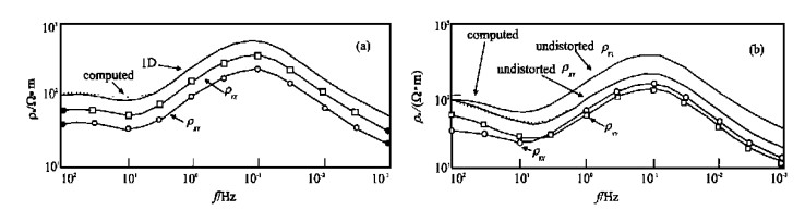
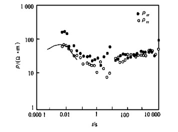
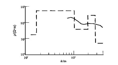
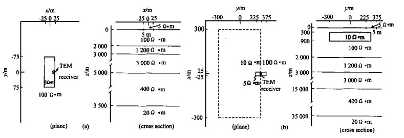
  • The inversion of TEM data, using the observed magnetic fields instead of that of apparent resistivities data in this paper, avoids the errors caused by the definition of the apparent resistivity. The inversed results by fitting the magnetic fields of the transmitter source's image with the observed magnetic fields are relatively less affected by the conductivity inhomogeneity. The MT apparent curve is calculated on the basis of the conductivity model constructed from the TEM inversion results. This curve is used as a reference curve for the correction of MT static shift, which makes the correction more reliable. Meanwhile, the domain transformation is also achieved from time to frequency between the two kinds of electromagnetic data. Therefore, the correction of the MT static shift is actualized using TEM inversion method. The corresponding application research shows that this method is very effective for the identification and correction of the MT static shift.


  • * This paper is supported by the previous Ministry of Coal Industry and Gansu Sciences Technology Committee.
  • The field and theoretical studies show that in the presence of near-surface inhomogeneities, MT apparent resistivity curves on the log apparent-resistivity versus log frequency display are always shifted in line with a factor, constant in all frequencies, with the impendence phase being unaffected, or with the static shift (Jones, 1988).

    It should be noted (Sternberg, 1988) that the parallel shift between two MT curves (TE and T M) at an MT site indicates these static shift effects.However, the absence of a displacement between these curves does not guarantee that there are static shifts.In general, the true resistivity may lie above, below, or between the curves from the two polarizations, or may agree with any one of the two polarization curves.The shifts are related to the boundaris of a surficial conductive inhomogeneity, to the direction of the boundary and to the distance between the boundary and the MT site.The T M mode is more sensitive to surficial charges.

    Previous work on MT static shift corrections falls roughly in the following six categories: (1) Spatial filtering method using closely-spaced MT sites, which is called electro-magnetic array profiling (EMAP) (Torres-verdin and Bostic, 1992). This method is effective for the static shift correction, but its cost is high.(2) Theoretical calculation of the static shift from buried-surface inhomogeneities (Wannamaker, 1984a).This method provides considerable physical insight into the static shift, but no sufficient information about the near-surface inhomogeneity can be obtained in advance, and the calculation is too expensive.(3) Theoretical calculation of the static shift from surface topographic effects (Wannamaker, 1986).This method is incapable of dealing with the static shift due to the subsurface bodies.(4) Interpretation based on known geology.(5) Direct correction of static shifts using inversion method (Meju, 1996; Ogawa and Uchida, 1996; de Groot-Hedlin, 1995, 1991).(6) Correction of static shifts by increasing the dipole length measuring electric field, by averaging local apparent resistivities, and by using the local high conductive layer.

    MT static shift is essentially a current channeling related to 3-D inhomogeneities, and the amount and direction of the shifts depend on the conductivity of the 3-D bodies.

    The difficulty in the calculation of MT is due to the unknown shape and position of the 3-D bodies, therefore, it is difficult to correct the static shifts by calculation of 3-D bodies (such as Wannamaker(1984a, b)).T raditional correction of static shifts is to locate an effective means to deal with the indefinite surface 3-D bodies.If there is no useful information, the correction of static shifts, which has been further developed by combining previous information obtained at surface, is to shift the doubtful apparent resistivity curve to a reference curve determined by some statistics or by some criteria (such as Jones (1988), Beamish and Travassos (1992)).However, in this case, an accurate correction of static shifts is hard to obtain. The work of Sternberg's (1988) and Pellerin and Hohmann's (1990) correction of MT static shifts using centra-l loop TEM apparent resistivities become a milestone, for they verified the effectiveness of the method, and made TEM soundings, globally popularized, a powerful means to interpret MT data in the depth of the earth.Since the TEM sounding, only used to measure the magnetic field, is not affected by the buildup of charges at the inhomogeneity boundaries (Sternberg, 1988), the effect of the surface inhomogeneity on the TEM curves is small and, therefore, the correction of static shifts by TEM soundings is considered as an effective means.Now this correction method, noted in China, has attracted many scholars and researchers, but the related reports are few and only limited to the correction of static shift using TEM apparent resistivity curves as reference.Furthermore, the accuracy in the calculation of the corresponding data is very difficult to obtain, for the definition of the TEM apparent resistivity is very complicated.The early or the late apparent resistivity, whose error is relatively large, is often used to make an approximate interpretation. Therefore, if TEM apparent resistivity is directly applied to the correction of MT static shifts, the unreliable results are bound to occur.In addition, in this correction method, the apparent resistivity in time-domain TEM sounding is transformed into that in frequency-domain, also resulting in some errors.In terms of the special effectiveness in the correction of MT static shifts using TEM technique without any aids of other information and also in terms of the need for the joint interpretation of multiple EM data, the authors have developed an approximate inversion of TEM data (Yang and Lin, 2000), where only the measured magnetic fields which are less affected by surface inhomogeneity, instead of apparent resistivities, were used for inversion. The TEM inversion results are used to create the model of the electrical structure whose MT apparent resistivity curve can be computed as a reference curve for correction, so that the identification and correction of MT static shifts can be actualized with TEM inversion.

    Both the forward and the inverse interpretations of models of the homogeneous half space and the layered earth are made in TEM, but the interpretation of the data from more complicated 2-D or 3-D models are more difficult to make, for the calculation of their responses are complicated and expensive.For the sake of simplification, based on the theories of smoke ring (Nabighian, 1979), people consider current lines in the earth, induced by transmitting source, as downward-moving and outward-expanding current filaments which are called as images of the source current.If the size, shape and magnetic moment of the images are thought of as the same as those of the transmitting source, the image depth can be determined by comparing the vertical magnetic field of the current filaments with that measured near the source.And then determined image depth can be used for the estimation of the downward vertical velocity of the image using a cubic spline interpolation method.Finally, the resistivities varying with depth can be approximately estimated through a comparison between the estimated velocity of the image and the downward diffusing velocity related to resistivities in a homogeneous half space (Eato and Hohmann, 1989). The centra-l loop TEM sounding technique is best adapted to the correction of MT static shifts because of its less sensitivity to the lateral resistivity variations than those of other TEM configurations (Nekut, 1987).

    In this paper, the measured magnetic fields, more reliable than the TEM apparent resistivities in characterizing the electrical structure of the subsurface, are used for inversion.But, usually, the measured data from the observation system are the partial derivatives of the magnetic field with respect to time.In addition, the magnetic fields are not directly given so that they must be estimated from the derivatives.The polynomial fitting shows that the measured derivatives range from the given latest delay time to a certain delay time at which the derivatives can be negligible.Then if the following formulation (Nekut, 1987) is used

    (1)

    H0 at the given latest delay time can be calculated.Finally, based on

    (2)

    the value of the magnetic field at any delay time during the observation can be obtained, which is also considered as the observed magnetic field.

    Because the measured responses are for 1-D layered or 2-D and 3-D models, it is necessary to obtain the image depth using the fitting approach where the configurations of multiple receiver with a single source are used.The fitting of the image with the measured fields is applied to the search for a minimum of their difference (Raiche and Galagher, 1985)

    (3)

    where N is the total number of receivers; Hzj(ti) is the vertical magnetic field measured at the jth receiver and Hzji (ti, d) is the vertical magnetic at the position of the jth receiver, owing to the image at the depth d beneath the source.

    After the position of the image at each discrete time has been determined, the next step is to estimate the resistivities and the depth to which each resistivity value corresponds.

    In a homogeneous half space, for a centra-l loop the diffusion velocity at the delay time t at the depth where the magnetic field's partial derivative is the maximum, i.e., at the penetration depth, is (Spies, 1989)

    (4)

    In (4), if the v is given, the resistivity can be estimated with the iterative fitting method.After the determination of the image position, i.e., the depth of the image, we can estimate the diffusion velocity at each delay time by using a cubic spline interpolation.It is difficult to derive the resistivity directly from the substitution of the estimated velocity for the corresponding variable in (4).When the iterative fitting method is employed, the apparent resistivity is substituted for the corresponding variable in (4) so as to obtain a velocity.Then this velocity is compared with the estimated velocity by a cubic spline interpolation in order to modify the resistivity.This comparison goes on until the fitting criterion is satisfied.Finally, using the empirical formulation, we can obtain the sounding depth

    (5)

    where 0.44 is an empirical constant.

    Based on the analysis above, we worked out an inversion program and tested it for the inversion of the 1-D theoretical models.The results show that the inversion effect is good (Yang and Lin, 2000).

    MT static shifts result from the distorted electrical field with the additional field yielded by the built-up electric charges, which do not affect the magnetic field, on the boundaries of near-surface heterogeneities.In addition, TEM soundings only measure the magnetic fields, but are not affected by the local near-surface heterogeneities.Sternberg (1988) reported that, when the delay time is later than 50 μs, the TEM apparent resistivity curve corresponding to the near-surface inhomogeneity is the same as that free of the anomaly.(In the following examples to be presented, the delay time of the data measured by the TEM instrument V5 ranges from 0.1063×10⁻³ s to 0. 8446×10-2 s so that the effect of near-surface inhomogeneity can be considered negligible).

    Therefore, the inversion results of the TEM data can be used as a reference to identify and correct MT static shifts.

    The size of the transmitting loop depends mainly on the TEM sounding depth, and does not greatly affect the sounding curves. However, a certain overlapped length between the TEM and the MT curves is required to correct MT static shifts. Therefore, a certain TEM sounding depth should occur to guarantee the effectiveness of the correction of static shifts.

    Spies (1989), who introduced a simple method to estimate the sounding depth in EM soundings, pointed out that the MT sounding depth depends mainly on the resistivities of the earth model and on the measured frequencies, and that the sounding depths, for the layered earth and a certain measuring system depend mainly on the average conductivity which is defined as the ratio of the integrated conductance to the total thickness of the model.The average conductivity calculated as a function of the depth can also be used approximately to estimate a lower limit of the inversion depth for layered models.In frequency domain, the sounding depth is about 1.5skin deep computed by the average conductivity and by the lowest frequency.In time domain, the sounding depth is about one diffusion depth computed by the average conductivity and by the latest delay time. In the same way, the smallest distinctive sounding depth can be estimated by the highest frequency in frequency domain or by the earliest delay time in time domain.However, above the smallest sounding depth, the conductivity thus determined is only an average conductivity.Therefore, the TEM sounding depth depends not only on the delay time and the resistivity, but also on the size of the transmitting loop expressed by its magnetic moment, and on the noise level (Spies, 1989)

    (6)

    In the following example, I is 7.5 A in (6);the area, A, of the loop is 100m×100m, and the average conductivity is 0.01 S/m, the estimated TEM sounding depth is about 1 000m, and the smallest MT sounding depth thus computed is about 350m.Therefore, there is a certain overlap, verified in the following context between the two sounding depths, and illustrating that the TEM data in the following examples can be used to correct the static shifts.

    When the obtained TEM data are transformed into the corresponding MT apparent resistivity curves, the TEM data is located in time domain and the MT data in frequency domain. In this case, the time-axis in TEM should be transformed into the corresponding frequency-or period-axis (Sternberg, 1988).

    MT skin depth is

    (7)

    TEM skin depth or penetration depth is

    (8)

    If δMTz, then

    (9)

    where f(Hz) refers to the measuring frequency; t (ms), the TEM delay time; 194, the constant which is called a conversion factor ranging from 150 to 200.In this paper, we use period T (s) instead of frequency f; delay time t with a unit s instead of ms, and the constant, 200. Then equation (9) can be changed into

    (10)

    There are two methods to identify and correct MT static shift.The first method is performed in the following steps: (1) The apparent resistivities are obtained from the computation of TEM inversion results, or the measured TEM apparent resistivities are directly used.(2) The time-axis of the TEM sounding curve is transformed into the corresponding frequency-axis by e-quation (9) or (10), and then the apparent resistivity curve in MT is compared with that in TEM for the identification of static shifts and the determination of the amount of the shifts.(3) MT static shifts are corrected.For the half-space model, this method is practical, but for the true earth model, transformation of the TEM sounding curve from the time domain to the frequency domain following equation (9) or (10) inevitably causes some errors.Therefore, the conversion factor in equation (9) or (10) should be determined in line with concrete conditions.The second correction method, especially when only the magnetic fields or their derivatives are given, is to draw up the layered earth model by TEM inversion results, and to compute the model's MT apparent resistivity curve which can be used as a reference curve to be compared with the measured MT apparent resistivity curve.In this way, the static shifts can be identified.If the overlaps show some obvious parallel displacements between the MT apparent resistivity curve derived from TEM inversion results and that of one or two polarization modes at the test site, the static shifts occur.Therefore, the correction factor can be determined from the amount of the parallel displacements so that the measured MT apparent resistivity curve is displaced to the reference curve.If no obvious displacement occurs, no static shifts may occur.In this paper, only the second method is used.It should be pointed out that the transformation from the TEM data in time domain to the MT data in frequency domain automatically comes true without the aid of equation (9) or (10). However, equation (9) or (10), based on the observation times in TEM soundings, can help us to estimate the frequency band of the MT curve of the model derived from the TEM inversion.In this case, more accurate MT curves can be obtained in more suitable frequency bands.

    Pellerin and Hohmann (1990) have corrected MT static shifts with centra-l loop TEM sounding technique, whose theoretical example is here introduced to illustrate its effectiveness. Figure 1a and 1b, respectively, denote the theoretical models with 1-D and 3-D near-surface inhomogeneity.Figure 2a and 2b present the diagrams for static-shift correction in the two models where the smooth curves represent the undistorted response, the dotted lines refer to computed MT reference curve to which the distorted ones will be shifted, and the circles and squares, respectively, refer to the distorted YX and XY polarization models of the apparent resistivity.In these figures, if both the distorted and undistorted curves are parallel to each other, there occurs an obvious static shift.The dotted line (serving as the reference curve) almost overlaps the undistorted curve at a high frequency band.Only parallel shifts to the reference curve serve as the terminals of the correction of static shifts, illustrating that the correction scheme obtained with the TEM technique works well.

    Figure  1.  Model of resistivity structure.(a).model1: a small (50m×150m×5m) conductive surficial inhomogeneity in a layered earth.The plane view shows the centra-l loop TEM receiver position; (b).model 2: a conductive surficial inhomogeneity and a large burried 3-D body in a layered earth.The layered earth and surficial body are as in (a).The stipped area represents a 10 Ω·m body embedded in the top 100 Ω·m layer.The TEM receiver location is centered on the surficial body (from Pellerin and Hohmann (1990)).
    Figure  2.  Diagram for static shift correction.The curves denoted by squares and circles are respectively the distorted responses for the XY and YX polarization modes and the dotted line represents the computed correction curve to which the distorted ones will be shifted.(a).for model1(solid line for the undistorted1-D response); (b).for model2(solid lines for the undistorted responses for two polarization modes) (from Pellerin and Hohmann (1990))

    Figure 3 shows the apparent resistivity curves of an MT sounding at Yuzhong Xiakou (E longitude 104°01.0′, N latitude35°49.0′), southeast of Lanzhou, in 1997.The Physical Prospecting Company, the First Exploring and Designing Institute, the Ministry of Railway, joined together to make a TEM sounding along a profile at the MT site using TEM instrument, V5, with a100 m ×100 m square loop, where the receiver is distributed along the line across the center of the loop.The current in the loop was 7.5A, and the delay times at the measured site changed from 0.1063×10⁻³ to 0.8446×10⁻² s with the fixed parameters of the measurement system.In order to test our program for TEM inversion, only the data at the square loop center can be used for the program work only on the condition of a circular loop.Since the magnetic field at the center of a square loop can be equivalent to that at the center of a circular loop with the same area, from πr2a2, i.e., raπ-1/2, the inversion scheme in the paper can be applied to the data at the center of the square loop.The inversion results thus obtained are in agreement with those of 1-D generalized inversion for TEM late-time field data (Yang and Lin, 2000).Correction of MT static shifts using TEM sounding technique must guarantee the same measurement position in the two EM soundings.Figure 4 shows the inversion results of the TEM data at such a position.The MT apparent resistivity curve computed for the model derived from the TEM inversion results is denoted by the solid line which can serve as a reference curve for the static-shift correction in Fig. 3 where the two observed MT curves at the measurement site are placed together for comparison.From Fig. 3, it can be seen that ρXY has a slight static shift, but ρYX hardly does.Comparing the reference curve with the measured data, one can determine the static shift factor which is about 0. 9 for ρXY, i.e., one can shift the ρXY multiplied by 0.9 to the reference curve.

    Figure  3.  MT apparent resistivity (solid line) computed by TEM inversion results and observed MT curves.
    Figure  4.  TEM inversion results at Yuzhong Xiakou.Solid line.inversion result in this paper; dash line.result by generalized inversion.

    It should be noted that only the apparent resistivities, but not the impedance phases, are affected by the static shift.Therefore, it is not necessary to correct for the phasesr (Jones, 1988).

    (1) In this paper, the identification and correction of the MT static shifts are introduced using TEM inversion where the derivatives of the measured magnetic fields are employed, instead of TEM apparent resistivities that have not been accurately defined.Therefore, the errors, caused by the TEM apparent resistivites in inversion, can be avoided.Meanwhile, the troubles of the conversion of the two EM data from time-to frequency-domain and errors caused by the conversion can also both be eliminated.

    (2) The inversion results by fitting the magnetic fields of the source image with the measured fields respond less to the surface inhomogeneity.In this case, the reference curves for MT static-shift correction derived from TEM inversion results become more reliable and the MT static shift correction also turns more reliable.

    (3) Compared with the correction scheme using joint inversion of TEM and MT data, the correction scheme involved in this paper has no necessity to choose which one of the two apparent resistivities will be applied to the inversion.

    (4) The real example shows that the static-shift correction scheme stated in this paper, simple, easy, practical and effective, can be made on a PC in no more than one minute.In addition, this static-shift correction scheme is convenient for the interpretation of the data in the field.

  • Beamish B, Travassos J M, 1992. A Study of Static Shift Removal from Magnetotelluric Data. J Appl Geophys, 29: 157-178 doi: 10.1016/0926-9851(92)90006-7
    de Groot-Hedlin G, 1991. Removal of Static Shift in Two Dimensions by Regularized Inversion. Geophysics, 56: 2102-2106 doi: 10.1190/1.1443022
    de Groot-Hedlin G, 1995. Inversion for Regional 2-D Resistivity Structure in the Presence of Galvanic Scatters. Geophys J Int, 122: 877-888 doi: 10.1111/j.1365-246X.1995.tb06843.x
    Eaton P A, Hohmann G W, 1989. A Rapid Inversion Technique for T ransient Electromagnetic Soundings. Phys Earth Planet Int, 53: 384-404 doi: 10.1016/0031-9201(89)90025-3
    Jones A G, 1988. Static Shift of Magnetotelluric Data and Its Removal in a Sedimentary Basin Environment. Geophysics, 53: 967-978 doi: 10.1190/1.1442533
    Lin C, Yang S, Ye J, 1994. One-Dimensional Inversion of TEM Late Time Field Data. Northwestern Seismological Journal, 16(2): 71 -78(in Chinese)
    Meju M A, 1996. Joint Inversion of TEM and Distorted MT Soundings: Some Effective Practical Considerations. Geophysics, 61: 56-65 doi: 10.1190/1.1443956
    Nabighian M N, 1979. Quas-i Static T ransient Response of a Conducting Half Space-An Approximate Respresentation. Geophysics, 44: 1700-1705 doi: 10.1190/1.1440931
    Nekut A G, 1987. Direct Inversion of Time-Domain Electromagnetic Data. Geophysics, 52: 1431-1435 doi: 10.1190/1.1442256
    Ogawa T, Uchida T A, 1996. Two-Dimensional Magnetotelluric Inversion Assuming Gaussian Static Shift. Geophys J Int, 126: 69-76 doi: 10.1111/j.1365-246X.1996.tb05267.x
    Pellerin L, Hohmann G W, 1990. T ransient Electromagnetic Inversion: A Remedy for Magnetotelluric Static Shifts. Geophysics, 55: 1242-1250 doi: 10.1190/1.1442940
    Raiche A P, Gallagher R G, 1985. Apparent Resistivity and Diffusion Velocity. Geophysics, 50: 1628-1633 doi: 10.1190/1.1441852
    Spies B R, 1989. Depth of Investigation in Electromagnetic Methods. Geophysics, 54: 872-888 doi: 10.1190/1.1442716
    Sternberg B K, 1988. Correction for the Static Shift in Magneto-Tellurics Using T ransient Electromagnetic Soundings. Geophysics, 53: 1459-1468 doi: 10.1190/1.1442426
    Torresverdin C, Bostic Jr F X, 1992. Principles of Spatial Surface Electric Field Filting in Magnetotelluric: Electromagnetic Array Profiling (EMAP). Geophysics, 97: 603-622
    Wannamaker P E, 1984a. Electromagnetic Modeling of T hree-Dimensional Bodies Using Integral Equations. Geophysics, 49: 60-74 doi: 10.1190/1.1441562
    Wannamaker P E, 1984b. Magnetotelluric Responses of T hree-Dimensional Bodies in Layered Earths. Geophysics, 49: 1517-1533 doi: 10.1190/1.1441777
    Wannamaker P E, 1986. Two-Dimensional Topographic Responses in Magnetotellurics Modeled Using Finite Elements. Geophysics, 51: 2131-2144 doi: 10.1190/1.1442065
    Yang C, Lin C, 2000. Approximate Inversion for3-D TEM Data. Acta Seismologica Sinica, 22(4): 377-384(in Chinese)
  • Relative Articles

    [1]Sixue Wang, Yong Zheng. Lithospheric reworking at the western margins of the Ordos Block Revealed by Joint inversion of Phase velocities and Receiver Functions[J]. Journal of Earth Science. doi: 10.1007/s12583-025-0242-1
    [2]Shuo Zhang, Jun Lu, Xiaobo Liu, Chengyu Pan, Zhidong Cai. Acoustic Full Waveform Inversion of DAS-VSP Data[J]. Journal of Earth Science, 2024, 35(5): 1795-1798. doi: 10.1007/s12583-024-0034-z
    [3]Junjie Wu, Xiaodong Chen, Yi Yang, Qingquan Zhi, Xingchun Wang, Jie Zhang, Xiaohong Deng, Yi Zhao, Yue Huang. Application of TEM Based on HTS SQUID Magnetometer in Deep Geological Structure Exploration in the Baiyun Gold Deposit, NE China[J]. Journal of Earth Science, 2021, 32(1): 1-7. doi: 10.1007/s12583-020-1086-3
    [4]Qingquan Zhi, Xiaohong Deng, Junjie Wu, Xiu Li, Xingchun Wang, Yi Yang, Jie Zhang. Inversion of IP-Affected TEM Responses and Its Application in High Polarization Area[J]. Journal of Earth Science, 2021, 32(1): 42-50. doi: 10.1007/s12583-020-1105-4
    [5]Zhanjun Xie, Xiangwen Liu, Zhenmin Jin, Zhuoyue Li. Microstructures and Phase Transition in Omphacite: Constraints on the P-T Path of Shuanghe Eclogite (Dabie Orogen)[J]. Journal of Earth Science, 2020, 31(2): 254-261. doi: 10.1007/s12583-019-1279-9
    [6]Jun Li, Chengli Liu, Yong Zheng, Xiong Xiong. Rupture Process of the Ms 7.0 Lushan Earthquake Determined by Joint Inversion of Local Static GPS Records, Strong Motion Data, and Teleseismograms[J]. Journal of Earth Science, 2017, 28(2): 404-410. doi: 10.1007/s12583-017-0757-1
    [7]Yi'an Cui, Zhixue Chen, Xiaoxiong Zhu, Haifei Liu, Jianxin Liu. Sequential and Simultaneous Joint Inversion of Resistivity and IP Sounding Data Using Particle Swarm Optimization[J]. Journal of Earth Science, 2017, 28(4): 709-718. doi: 10.1007/s12583-017-0749-1
    [8]Kaiming Li, Zhongqin Li, Cuiyun Wang, Baojuan Huai. Shrinkage of Mt. Bogda glaciers of eastern Tian Shan in Central Asia during 1962–2006[J]. Journal of Earth Science, 2016, 27(1): 139-150. doi: 10.1007/s12583-016-0614-7
    [9]Jan van der Kruk, Nils Gueting, Anja Klotzsche, Guowei He, Sebastian Rudolph, Christian von Hebel, Xi Yang, Lutz Weihermüller, Achim Mester, Harry Vereecken. Quantitative multi-layer electromagnetic induction inversion and full-waveform inversion of crosshole ground penetrating radar data[J]. Journal of Earth Science, 2015, 26(6): 844-850. doi: 10.1007/s12583-015-0610-3
    [10]Runhai Feng, Ping Dong, Liangshu Wang, Bin Sun, Yongjing Wu, Changbo Li. Inversion of Moho Interface in Northeastern China with Prior Information[J]. Journal of Earth Science, 2014, 25(1): 146-151. doi: 10.1007/s12583-014-0407-9
    [11]Guiju Wu, Xiangyun Hu, Guangpu Huo, Xiaochen Zhou. Geophysical Exploration for Geothermal Resources: An Application of MT and CSAMT in Jiangxia, Wuhan, China[J]. Journal of Earth Science, 2012, 23(5): 757-767. doi: 10.1007/s12583-012-0282-1
    [12]Ningning Zhang, Yuanqing He, Wilfred H Theakstone, Hongxi Pang. Chemical Composition of Aerosol and Fresh Snow and Tourism Influences at Baishui Glacier No. 1 from Mt. Yulong, Southeastern Tibetan Plateau[J]. Journal of Earth Science, 2010, 21(2): 199-209. doi: 10.1007/s12583-010-0018-z
    [13]Huan Yang, Weihua Ding, Gangqiang He, Shucheng Xie. Archaeal and bacterial tetraether membrane lipids in soils of varied altitudes in Mt. Jianfengling in South China[J]. Journal of Earth Science, 2010, 21(S1): 277-280. doi: 10.1007/s12583-010-0235-5
    [14]Fengli Yang, Haixiao Yu, Qinglin Zhang, Qianyu Li. Correlations between Shortening Rate, Uplift Rate, and Inversion Rate in Central Inversion Zone of Xihu Depression, East China Sea Basin[J]. Journal of Earth Science, 2009, 20(4): 699-708. doi: 10.1007/s12583-009-0056-6
    [15]Ugur Yaramanci, Mike Müller-Petke. Improvements in Inversion of Magnetic Resonance Exploration—Water Content, Decay Time, and Resistivity[J]. Journal of Earth Science, 2009, 20(3): 592-605. doi: 10.1007/s12583-009-0049-5
    [16]Yuan-qing HE, Zong-sheng LI, Xiao-mei YANG, Wen-xiong JIA, Xian-zhong HE, Bo SONG, Ning-ning ZHANG, Qiao LIU. Changes of the Hailuogou Glacier, Mt. Gongga, China, against the Background of Global Warming in the Last Several Decades[J]. Journal of Earth Science, 2008, 19(3): 271-281.
    [17]Hanlie Hong, Xiaoling Zhang, Miao Wan, Yijun Hou, Dengwen Du. Morphological Characteristics of (K, Na)-Rectorite from Zhongxiang Rectorite Deposit, Hubei, Central China[J]. Journal of Earth Science, 2008, 19(1): 38-46.
    [18]Sheng JIN, Gao-feng YE, Wen-bo WEI, Ming DENG, Jian-en JING. Electrical Structure and Fault Features of Crust and Upper Mantle beneath the Western Margin of the Qinghai-Tibet Plateau: Evidence from the Magnetotelluric Survey along Zhada-Quanshui Lake Profile[J]. Journal of Earth Science, 2007, 18(4): 326-333.
    [19]Bai-yao RUAN, Shi-zhe XU, Zhi-feng XU. Modeling the 3D Terrain Effect on MT by the Boundary Element Method[J]. Journal of Earth Science, 2006, 17(2): 163-167.
    [20]Handong Tan, Sheng Jin, Wenbo Wei, Leshou Chen, Ming Deng. Electrical Structure of Yarlung Zangbo Suture from Magnetotelluric Profiling of INDEPTH-MT[J]. Journal of Earth Science, 2000, 11(3): 325-327.
  • Created with Highcharts 5.0.7Amount of accessChart context menuAbstract Views, HTML Views, PDF Downloads StatisticsAbstract ViewsHTML ViewsPDF Downloads2024-062024-072024-082024-092024-102024-112024-122025-012025-022025-032025-042025-0502468
    Created with Highcharts 5.0.7Chart context menuAccess Class DistributionFULLTEXT: 49.0 %FULLTEXT: 49.0 %META: 49.0 %META: 49.0 %PDF: 2.0 %PDF: 2.0 %FULLTEXTMETAPDF
    Created with Highcharts 5.0.7Chart context menuAccess Area Distribution其他: 1.5 %其他: 1.5 %China: 43.5 %China: 43.5 %Japan: 2.5 %Japan: 2.5 %Korea Republic of: 1.5 %Korea Republic of: 1.5 %Reserved: 3.0 %Reserved: 3.0 %Russian Federation: 18.0 %Russian Federation: 18.0 %Singapore: 1.0 %Singapore: 1.0 %United States: 29.0 %United States: 29.0 %其他ChinaJapanKorea Republic ofReservedRussian FederationSingaporeUnited States

Catalog

    通讯作者: 陈斌, bchen63@163.com
    • 1. 

      沈阳化工大学材料科学与工程学院 沈阳 110142

    1. 本站搜索
    2. 百度学术搜索
    3. 万方数据库搜索
    4. CNKI搜索

    Figures(4)

    Article Metrics

    Article views(97) PDF downloads(4) Cited by()
    Proportional views
    Related

    /

    DownLoad:  Full-Size Img  PowerPoint
    Return
    Return