Processing math: 100%
Advanced Search

Indexed by SCI、CA、РЖ、PA、CSA、ZR、etc .

Limei Wang, Guowang Jin, Xin Xiong. Flood Duration Estimation Based on Multisensor, Multitemporal Remote Sensing: The Sardoba Reservoir Flood. Journal of Earth Science, 2023, 34(3): 868-878. doi: 10.1007/s12583-022-1670-9
Citation: Limei Wang, Guowang Jin, Xin Xiong. Flood Duration Estimation Based on Multisensor, Multitemporal Remote Sensing: The Sardoba Reservoir Flood. Journal of Earth Science, 2023, 34(3): 868-878. doi: 10.1007/s12583-022-1670-9

Flood Duration Estimation Based on Multisensor, Multitemporal Remote Sensing: The Sardoba Reservoir Flood

doi: 10.1007/s12583-022-1670-9
More Information
  • Corresponding author: Guowang Jin, guowang_jin@163.com
  • Received Date: 21 Dec 2021
  • Accepted Date: 09 Apr 2022
  • Issue Publish Date: 30 Jun 2023
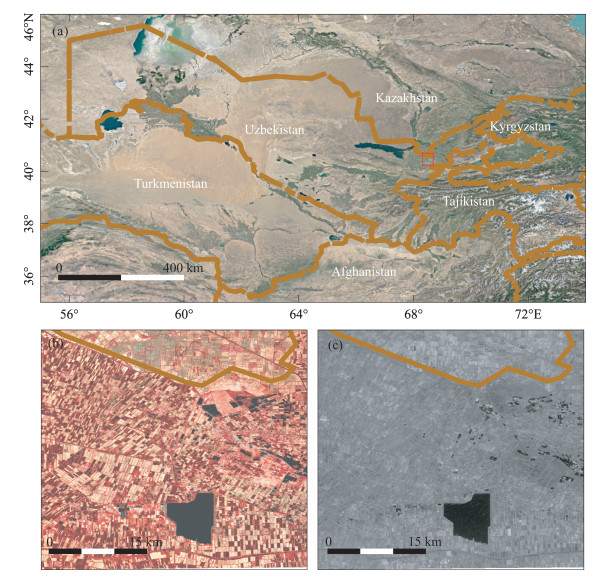
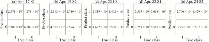
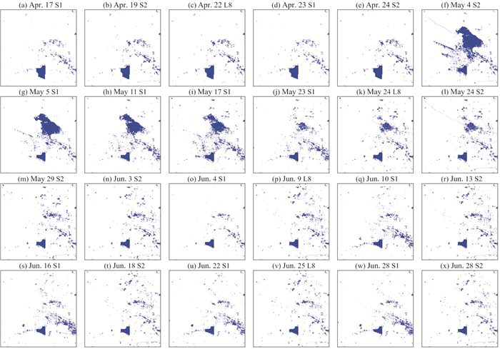
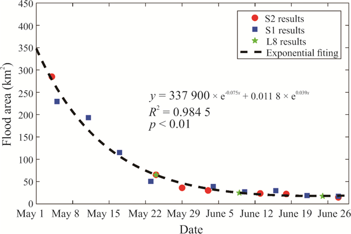
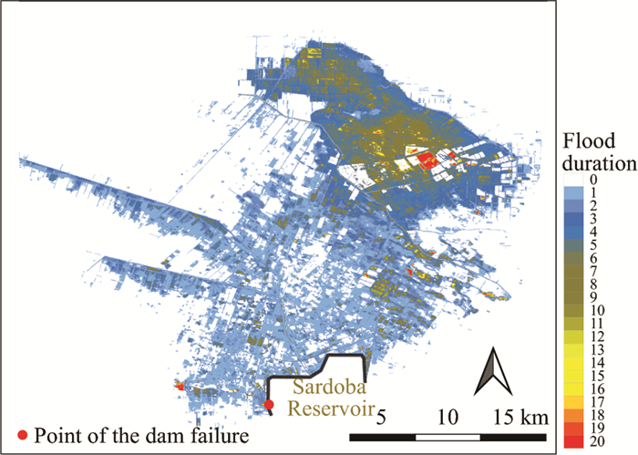
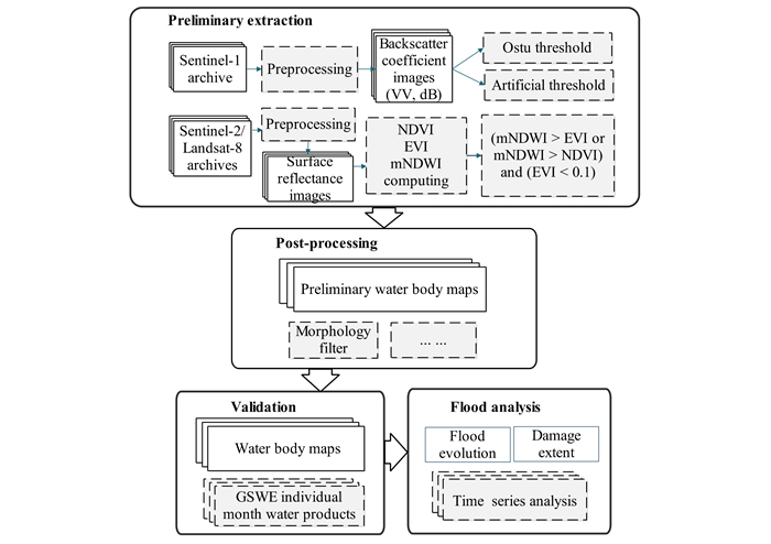
  • Single-sensor monitoring of flood events at high spatial and temporal resolutions is difficult because of the lack of data owing to instrument defects, cloud contamination, imaging geometry. However, combining multisensor data provides an impressive solution to this problem. In this study, 11 synthetic aperture radar (SAR) images and 13 optical images were collected from the Google Earth Engine (GEE) platform during the Sardoba Reservoir flood event to constitute a time series dataset. Threshold-based and indices-based methods were used for SAR and optical data, respectively, to extract the water extent. The final sequential flood water maps were obtained by fusing the results from multisensor time series imagery. Experiments show that, when compare with the Global Surface Water Dynamic (GSWD) dataset, the overall accuracy and Kappa coefficient of the water body extent extracted by our methods range from 98.8% to 99.1% and 0.839 to 0.900, respectively. The flooded extent and area increased sharply to a maximum between May 1 and May 4, and then experienced a sustained decline over time. The flood lasted for more than a month in the lowland areas in the north, indicating that the northern region is severely affected. Land cover changes could be detected using the temporal spectrum analysis, which indicated that detailed temporal information benefiting from the multisensor data is highly important for time series analyses.


  • In arid Central Asia, several large reservoirs have been built along rivers to support agricultural irrigation and daily water consumption. However, this construction has had a substantial impact on the local ecological environment and increases the risk of flooding (Criss, 2016; Duan et al., 2016). Dynamic monitoring of flood events using satellite observation data is an important tool for protecting the regional climate, security, and environment (Pandey et al., 2021; Voigt et al., 2016). Multispectral remote sensing data (typically Moderate Resolution Imaging Spectroradiometer (MODIS), Landsat, and Sentinel-2 series data) are mostly used for flood detection (Yang et al., 2020; Tulbure et al., 2016). Given the limitations of optical imagery for high-frequency flood monitoring, the utilization of synthetic aperture radar (SAR) is an important development (Amitrano et al., 2018).

    Numerous methods have been developed for floodwater detection, including threshold-based methods (Fang et al., 2011), indices-based methods (Feyisa et al., 2014), spectral angle distance (Shah-Hosseini et al., 2015), classification-based methods (Verpoorter et al., 2014), and other advanced techniques (Yang and Chen, 2017). Water and vegetation indices, such as the normalized difference water index (NDWI), modified NDWI (mNDWI), normalized difference vegetation index (NDVI), and enhanced vegetation index (EVI) are mostly used for multispectral optical images (Deo et al., 2018). Setting threshold values for HH (horizontal transmission and horizontal reception), HV (horizontal transmission and vertical reception), VV (vertical transmission and vertical reception), and VH (vertical transmission and horizontal reception) backscatter coefficients (BC) is a common method for SAR-based flood detection (Li and Wang, 2015; Refice et al., 2014). Further, k-means clustering, k-nearest neighbors, support vector machines, random forest classifiers, and deep learning frameworks are consistently used in flood monitoring (Pickens et al., 2020; Sarker et al., 2019).

    Currently, flood monitoring relies mainly on single-sensor data. Owing to the limitations caused by the revisit period, spatial resolution, cloud contamination, and other factors (Tholey et al., 2015; Chaouch et al., 2012), single-sensor data cannot provide detailed information on flood development. The problem is worsened by the typically cloudy, windy, and rainy weather conditions associated with flood events, which hinder the propagation of waves in the optical spectral range and thereby impede acquisitions by optical sensors. This problem is not present for longer wavelengths; therefore, SAR imaging sensors represent workable solutions for long-term flood event monitoring. The stack of multisensor images constitutes a special solution for ensuring a deep understanding of flood events (Refice et al., 2018). The integration of multisensor data (i.e., SAR and optical sensors) overcomes the disadvantages of single-sensor data, increases the revisit frequency, and provides multidimensional features to improve the accuracy and reliability of flood monitoring (D'Addabbo et al., 2016).

    The Google Earth Engine (GEE) provides us with a cloud computing platform supported by various geospatial datasets, including satellite imagery, aerial imagery, shuttle radar topography mission (SRTM) global digital elevation model (DEM), precipitation, wind, and other auxiliary data. Many satellite datasets such as Landsat Thematic Mapper (TM), Enhanced Thematic Mapper Plus (ETM+), Operational Land Imager (OLI), Sentinel-1 (S1), and Sentinel-2 (S2) can be easily collected and used in GEE, which is highly important in multisensor and multitemporal applications (Tamiminia et al., 2020). In addition, many modules, algorithms, and functions that can process large-scale data for various applications are provided by the GEE. Based on its powerful cloud computing capability, new ideas or algorithms can be implemented.

    The Sardoba Reservoir was built entirely on the plain, using only a very limited slope. So it had to be built on three sides, rather than just one side, as in the case of river closure. This was not only costly but also increased the risk of leaks due to the length of the dam. On May 1, 2020, the Sardoba Reservoir burst after heavy rain and strong winds, causing severe damage to nearby residential areas, farmland, and communication facilities. It was reported that the burst may be directly related to the contact leakage of a 29-meter-high water conveyance structure (i.e., the culvert pipes through the dam) and it happened in an instant. The reservoir was nearly full of waters when it burst. The outburst flood not only affected Uzbekistan itself but also parts of neighboring Kazakhstan. According to the report, there were problems with the dam's design, construction and operation, which ultimately led to the dam failure.

    In the Sardoba Reservoir flood cases, cloudy and rainy weather conditions were common in the two months before and after the flood event (from April to May 2020); consequently, more than 60% of the optical imagery was polluted by clouds (> 20%). Only in June 2020, approximately 20 percent of the optical imagery was polluted. In this research, 6 optical-sensor images were excluded because of extensive clouds, and 13 images were chosen from two optical sensors (i.e., Landsat-8 (L8) and Sentinel-2) that completely covered the study area. Integrating with 11 Sentinel-1 images, a sequential stack of 24 images was built to explore the performance of this configuration in the selected flood event (Table 1). We focus on addressing the following questions.

    Table  1.  Time series dataset composed of three sensors' images (i.e., Landsat-8, Sentinel-2, Sentinel-1)
    Sequence No Landsat-8 Sentinel-2 Sentinel-1
    1 April 17, 2020
    2 April 19, 2020
    3 April 22, 2020
    4 April 23, 2020
    5 April 24, 2020
    6 May 4, 2020
    7 May 5, 2020
    8 May 11, 2020
    9 May 17, 2020
    10 May 23, 2020
    11, 12 May 24, 2020 May 24, 2020
    13 May 29, 2020
    14 June 3, 2020
    15 June 4, 2020
    16 June 9, 2020
    17 June 10, 2020
    18 June 13, 2020
    19 June 16, 2020
    20 June 18, 2020
    21 June 22, 2020
    22 June 25, 2020
    23, 24 June 28, 2020 June 28, 2020
     | Show Table
    DownLoad: CSV

    (1) How does the accuracy of water body extraction using SAR and optical satellite imagery compare with the reference maps?

    (2) What advantages do the combined multisensor data entail for time series analyses of flood monitoring, especially in terms of providing detailed information to ensure a better understanding of flood events?

    (3) How does temporal information benefiting from the multisensor data act in detecting land surface changes caused by the flood development?

    Figure 1 shows the flow chart of this study. Figure 2 shows the location of the study area. Figure 3 and Table 1 show the time series dataset used in this study; the dataset is composed of the imagery from Landsat-8, Sentinel-1, and Sentinel-2. The images are arranged in a temporal sequence in Fig. 3 and Table 1; note that two images were obtained from different sensors respectively on May 24 and June 28, 2020. All images entirely cover the area of interest (red rectangle in Fig. 2).

    Figure  1.  Flow chart of this study.
    Figure  2.  Maps showing the location of the study area (a) near the Uzbekistan-Kazakhstan border (dashed line), along with detailed Sentinel-2 (b) and Sentinel-1 (c) images of the region near the Sardoba Reservoir (black).
    Figure  3.  A time series dataset composed of multisensor images for flood monitoring (i.e., Sentinel-1 (S1), Sentinel-2 (S2), and Landsat-8 (L8)). All optical images use SWIR-red-green as R-G-B.

    Uzbekistan, one of the five Central Asian counties, is located in the central part of the region. It is a dual-landlocked country with a typical continental climate with severe drought. Precipitation is concentrated in the winter and spring seasons, with less than 200 mm in lowland plains and approximately 1 000 mm in mountainous areas. The lowland plains, most of which are located in the Kizilkum Desert in the northwest, account for 80% of the total area. Ten percent of the country's area is covered by intensive arable lands, canals, and valleys. Developed agriculture is one of the country's major industries, as Uzbekistan is the world's sixth-largest cotton producer and second-largest cotton exporter. Owing to perennial drought and water shortages, water conservancy infrastructure for irrigated agriculture is highly developed, supporting an area of 4.25 million hectares of irrigated lands.

    The Sardoba Reservoir was built in 2017 in the eastern region of Uzbekistan which is one of the five Central Asian counties located in the central part of the Central Asian region. The Sardoba Reservoir has a maximum storage capacity of 920 million cubic meters (Fig. 2), which is surrounded by a large number of cultivated lands and is mainly used for agricultural irrigation. The Sardoba Reservoir is one of several reservoirs built along the Syr River which is one of the main inland rivers in Uzbekistan. It relies on water diversion and injection and is built entirely on plain terrain making limited use of the topographical slope. On May 1, 2020, the Sardoba Reservoir burst after a heavy storm. The water soon spilled to the north, inundating villages and farmlands around the reservoir. Because it was built on a narrow finger of land in Uzbekistan, the water rushed across the border, inundating parts of Kazakhstan as well. This flood caused severe damage to nearby settlements, farmlands, and communication facilities. After the accident, approximately 70 000 persons were evacuated, 2 children were killed, and 56 persons were hospitalized.

    Landsat-8 data collection includes the atmospherically corrected surface reflectance. These images contain five visible and near-infrared bands, two short-wave infrared bands processed to orthorectified surface reflectance, and two thermal infrared bands processed to orthorectified brightness temperature (Young et al., 2017).

    Under the limitation of a 16-day revisit cycle for the Landsat satellite missions, Landsat-8 OLI surface reflectance images corresponding to five scenes in the study area were collected from the GEE from April 17 to June 28, 2020 (Table 1). By excluding one scene covered by extensive clouds, only four cloud-free scenes were used to detect the flood event (Fig. 3). During image preprocessing, radiation correction, atmospheric correction, orthorectification, and cross-calibration among the different sensors (Dwyer et al., 2018; Wudler et al., 2015) were performed.

    Sentinel-1 carries a dual-polarization C-band SAR instrument operating at a center frequency of 5.405 GHz and containing 4 exclusive instrument modes with different swatch widths and spatial resolutions. The Interferometric Wide (IW) mode, which combines a large swath width (250 km) with a moderate geometric resolution (5 m × 20 m), is the default and primary acquisition mode over land and is expected to achieve a high resolution and potentially global coverage over landmasses. A single Sentinel-1 satellite can map the world once every 12 d. Sentinel-1A and Sentinel-1B share the same orbit plane with a 180° orbital phasing difference. The repeat cycle was 6 d when both satellites were in operation. The Sentinel-1 mission currently provides the only open SAR satellite data that can be freely downloaded.

    Sentinel-1 ground range detected (GRD) data is a collection of BC images that is updated daily. Each scene of the collection has one of three resolutions (10, 25, or 40 m), three instrument modes, and four polarization band combinations (VV or HH or VV + VH or HH + HV). Sentinel-1 GRD data collection was performed with the Sentinel-1 toolbox on the GEE using the following steps: thermal noise removal, speckle noise removal, radiometric calibration, and terrain correction using SRTM DEM or ASTER DEM for areas with a latitude greater than 60° where SRTM is not available. The final terrain-corrected values are converted to BC in decibels via log scaling (i.e., 10 × log10 (x)). The BC images were then precisely geocoded using the Range-Doppler algorithm (Kay et al., 2003) and resampled to a 20 m × 20 m resolution.

    Eleven scenes of Sentinel-1 GRD data corresponding to the study area, as observed by dual-polarization bands (VV + VH) in the IW mode, were used to detect the flood event (Table 1, Fig. 3); the data were obtained from the GEE from April 17 to June 28, 2020, and two scenes were abandoned for the radiation distortion of water surface caused by the heavy wind.

    Sentinel-2 is a wide-swath, high-resolution, multispectral imaging (MSI) mission composed of two optical satellites A and B with a 5-day revisit cycle of the constellation. The satellites provide 13 bands, including visible light, near-infrared, and short-wave infrared, with obvious advantages in terms of both spectral and spatial resolutions compared to the corresponding spectral range of Landsat missions; these tools support the monitoring of vegetation, soil, and water cover, as well as observations of inland waterways and coastal areas (Pasqualotto et al., 2019).

    The Sentinel-2 data contains the level-2A bottom of atmosphere (BOA) reflectance in the cartographic geometry mode. It was generated from level-1C data using sen2cor by radiation calibration and atmospheric correction. Nine scenes of Sentinel-2 BOA data of the study area collected from the GEE from April 17 to June 28, 2020, were used to detect the flood event, and five scenes were abandoned (Table 1, Fig. 3). All optical images used here were not processed via cloud removal and interpolation. The images with extensive clouds were abandoned in our study, thereby ensuring the reliability of the findings and accuracy of the pixel-level time series analysis.

    The mNDWI, EVI, and NDVI were used to build a classification tree for extracting the water body pixels (Panetti et al., 2012). Three indices of each pixel were calculated separately for the Landsat-8 and Sentinel-2 surface reflectance images using the spectral bands and equations listed in Table 2. The pixels whose water signal was stronger than the vegetation signal were classified as open-surface water bodies using the criterion mNDW > EVI or mNDWI > NDVI. To further remove the mixed pixels of water and vegetation, EVI < 0.1 was used as the criterion to remove the vegetation noise. Therefore, classification criteria of (mNDWI > EVI or mNDWI > NDVI) and (EVI < 0.1) were used to distinguish the water body pixels from the non-water pixels. The algorithms were proposed and verified using millions of Landsat images on the GEE platform (Zou et al., 2018, 2017). To reduce the small-size pseudo-water pixels caused by the radiated noise, a focal-mode morphology filter was used to generate the final flood maps for each date, which were formed by an octagon-shaped kernel with a 10-pixel radius.

    Table  2.  Datasets and methods used in this study
    Dataset Resampled resolution Parameters Methods Purpose
    Landsat-8 OLI surface reflectance
    Sentinel-2 MSI surface reflectance
    20 m mNDWI=ρGreenρSWIRρGreen+ρSWIRNDVI=ρNIRρRe dρNIR+ρRe dEVI=2.5×(ρNIRρRe d)1.0+ρNIR+6.0×ρRe d+7.5×ρBlue (mNDW > EVI or mNDWI > NDVI) and EVI < 0.1 Producing binary water body maps
    Sentinel-1 GRD 20 m Backscatter coefficient of VV polarization in decibels via log scaling 10×log10(x) Otsu threshold; artificial threshold Producing binary water body maps
    GSWD 20 m Individual month water percent map Accuracy assessment of binary water maps
     | Show Table
    DownLoad: CSV

    Otsu algorithm automatically calculates and determines the threshold for dividing water body and non-water body by seeking the maximum variance in the statistical results of pixel gray values. Therefore, when there is an obvious gap between the gray values of the water body and the non-water body in the SAR image, that is when the frequency distribution of the gray value of the SAR image has obvious 'peak-valley' characteristics, the Otsu algorithm has high water body extraction accuracy. And the larger the difference between peak and valley, the better the segmentation effect (Cao et al., 2017). For SAR images with two peaks in the frequency distribution histogram (i.e., bimodal images), the optimal threshold obtained by the Otsu algorithm is approximately equal to the valley between the two peaks. However, the accuracy of the Otsu algorithm is limited when the gap between two peaks of a SAR image is not obvious (i.e., non-bimodal images). The Otsu algorithm can be formulated as follows.

    σ2=p1p2(m1m2)2 (1)
    p1=ki=0pi,p1+p2=1 (2)
    m1=1/p1×ki=0ipi (3)
    m2=1/p2×L1i=k+1ipi (4)

    where σ2 is the interclass variance, m1, m2 is the mean value of each category, p1, p2 is the probability, and the pixel value k that maximizes Eq. (1) is the required Otsu threshold.

    In this study, flood extraction based on the Otsu algorithm was conducted on Sentinel-1 VV BC images as follows: a focal median filter was applied to reduce the speckle noise of SAR images, the histogram of each image was calculated, and the Otsu threshold was implemented to generate the preliminary water body maps. For non-bimodal SAR images, the results obtained using the Otsu algorithm may be unsatisfactory. In this case, we used the empirical threshold method to extract water bodys based on visual analysis. Then, morphological filtering was used to remove small pseudo water pixels caused by the remaining speckle noise and other factors to obtain the final water body maps.

    The Global Surface Water Dynamic (GSWD) dataset (https://glad.umd.edu/dataset/global-surface-water-dynamics) was used to evaluate the accuracy of water extent detection using our methods. The GSWD maps were generated from all Landsat-5, 7, and 8 data from 1999 to 2020 (Pickens et al., 2020). The maps contain 10° × 10° tiles of five layers, and the layer corresponding to monthly water percentage was used to perform a comparison with our water maps. Because the flood event was not captured by the GSWD, the accuracy evaluation of the flooded area was not possible. As an alternative, the water maps extracted from three sensors (i.e., S1, S2, and L8) in April 2020 before the flood event were compared with the corresponding GSWD water percentage map (Fig. 4).

    Figure  4.  Comparison of water extraction results from multisensor imagery sensed in April 2020, where (a) is the GSWD water map in April 2020, (b)–(f) are water extraction results using our methods.

    The confusion matrixes were subsequently obtained (Fig. 5). Five indicators were then calculated based on the confusion matrix to quantitatively evaluate the accuracy of the water extraction results: producer accuracy (PA), user accuracy (UA), overall accuracy (OA), kappa coefficient (Kappa), and F1-score. Larger values of the five parameters indicate superior accuracy. The results (Table 3) show that the OAs were about 99% for all waterbody maps. In general, the water extents predicted by our methods are highly accurate but smaller than those of the reference map. Similarly, the S1-predicted water extents are smaller than those of S2 and L8, with the latter two showing similar results.

    Figure  5.  The confusion matrixes of the water extraction results in this study. '1' represents the water body category and '0' represents the non-water body category.
    Table  3.  Comparison between produced water body maps and GSWD product
    Predicted water body maps PA (%) UA (%) OA (%) Kappa F1-score
    Apr. 17 Sentinel-1 78.3 95.3 98.8 0.854 0.860
    Apr. 23 Sentinel-1 77.9 92.5 98.7 0.839 0.846
    Apr. 19 Sentinel-2 86.7 91.3 99.0 0.884 0.889
    Apr. 24 Sentinel-2 82.5 95.0 99.0 0.878 0.883
    Apr. 22 Landsat-8 85.9 95.3 99.1 0.900 0.903
     | Show Table
    DownLoad: CSV

    Threshold-based and indices-based classification methods were applied to 11 SAR images and 13 optical images, respectively, to extract the water body maps from April 17 to June 28, 2020, as shown in Fig. 6. A total of 24 binary maps were generated, in which the value of 1 represented water pixels and 0 represented non-water pixels. In addition, the flood areas for each date were calculated during the flood period, as shown in Fig. 7.

    Figure  6.  Binary water body maps derived from multisensor imagery (i.e., L8, S1, S2) during the flood period, shown in temporal sequence. The white region (with the pixel value of 1) represents the water pixels, whereas the black area (with the pixel value of 0) represents the non-water pixels.
    Figure  7.  Temporal change in total water body area during the whole flooding period as predicted by the multisensor imagery.

    Figure 6 show that the floodwater arrived in the northernmost areas before May 4, three days after the flood event occurred, indicating that the floodwater moved rapidly. Extensive areas of farmlands and villages were flooded. For the lowland areas in the north, the floodwater lasted for more than a month and then completely receded around June 10. However, continual changes in land surface features can still be seen in the sensed images after the flood, showing the long-duration damage of this disaster. Figure 7 shows that the water area was stable before the flood, and the numeric values calculated from the multisensor images are in accordance. An abrupt change in water body area can be observed by Fig. 7 on May 1 when the flood occurred. The water body area arrived at its maximum between May 1 and May 4 and then experienced a sustained decline along with the time.

    We calculated the flooded area for each date and observed notable changes during the flood period, as shown in Fig. 8. The graph shows that the flooded area increased sharply to a maximum before May 4 according to the regression analysis. It then experienced a sustained decline along with the flood development. Around June 26, the flooded area became next to nil, indicating the disappearance of the floodwater.

    Figure  8.  Change in the flooded areas during the flood development.

    Flood development could be tracked using a sequence map fused by 24-date water body maps generated from SAR and optical imagery. For each pixel, we counted the number of dates that 1 was present in the 24 binary maps and recorded the dates, ultimately fusing them into a sequence map (Fig. 9). Different colors on the map indicate the duration of floodwater and the damage extent. Time series data composed of multisensor images offer an effective tool for tracking this flood event at high temporal resolution. For example, Fig. 9 shows that the regions where the duration of floodwater lasted more than 10 days were concentrated northeast of the study area, indicating severer damage in those areas. In addition, some regions in the northeast were flooded for more than a month.

    Figure  9.  A sequence map of the floodwater fused by all results from multisensor imagery. Different colors indicate the extent and the duration of the flooding.

    As we all know, water pixels have both low SAR BC and high mNDWI values, which help us distinguish water from other land cover classes. Once a region is flooded, it will be dominated by water's signature in remote sensing images and derived feature maps. During a flood event, land surface change is mainly manifested as the transition between the water bodies and other land types, and such change information can be found and extracted by time trajectory analysis of the spectral characteristics. The duration of a flood can also be estimated by time trajectory analysis. We selected 4 sites to analyze the temporal changes in land surface features (i.e., SAR BC and mNDWI) caused by the flood event. The sites were labeled as P1, P2, P3, and P4, which represent the permanent water of the reservoir, the retreat of the reservoir, the flooded area, and the permanent land, respectively. The locations of the 4 sites were marked on a Sentinel-1 image sensed on May 4, 2020 (Fig. 10c). For each site, we extracted the values of the BC and mNDWI for each date from the SAR BC and optical mNDWI maps, respectively. These are plotted in the graphs shown in Fig. 10. The graph shows different patterns of the land surface change for the four tested sites, from which abrupt change points can be found during the flood period. Figure 10 showed that P3 (shown in red) exhibited a sudden change in pixel values (i.e., BC and mNDWI) on May 4th and then recovered on May 24th; this indicated that P3 had been flooded during May 4–24. Similarly, P2 (shown in light blue) suddenly changed its BC and mNDWI values on May 4th and never changed back. In contrast, there was no significant variation found in BC and mNDWI values of P4 (shown in green) throughout the flood period, indicating it was not affected by this flood.

    Figure  10.  Time trajectory analysis of (a) backscatter coefficient and (b) mNDWI index during the flood, (c) location of the selected 4 sites used to analyze the temporal changes in land surface featuresmarked on a Sentinel-1 image sensed on May 4, 2020.

    It's worth noting that, both the BC and mNDWI values of P1 (shown in blue) showed obvious fluctuation during the flood period. Based on the literature (Lu et al., 2017; Yu et al., 2009), we tend to attribute the mNDWI's fluctuation to the spectrum variation of water body in S2 and L8 images caused by the water depth changes due to factors such as flood and wind. Lu et al. (2017) state that water depth is highly correlated with the spectrum in the visible region, and the maximum correlation value reached at 550 nm (i.e., the green band). The water index (i.e., mNDWI) is calculated by the green band and short-wave infrared band. Therefore, we deduced that water depth is the key factor for the fluctuation of mNDWI. Similarly, wind and water depth can change the water body's spectral response to the microwave band, which causes the fluctuation of the water body's BC in SAR images. It should be noted that although the BC and mNDWI of water bodies fluctuate to some extent, these two parameters are still capable to distinguish water bodies from other land covers, which can be proven from Fig. 10.

    Time series data can help us understand biological and environmental dynamics. The sudden occurrence of environmental and disaster events caused by climate change and human activities are increasing. These events may happen fast or last for a few days, weeks, or months. Extremely high spatial and temporal resolutions are key to detecting and tracking the development trends of these events. However, single-sensor products cannot offer high spatial, spectral, and temporal resolutions. To yield an acceptable spatial resolution, sensors must possess pixels of a smaller size, resulting in a narrower swath width; this leads to a long revisit cycle of many days, and thus, a lower temporal resolution (Ban and Jacob, 2013). Employing a sequence of multisensor images constitutes a special solution to this problem. The revisit interval of Landsat-8 (30-m spatial resolution) was 16 d, that of Sentinel-1 (double satellites) was approximately 6 d, and that of Sentinel-2 (double satellites) was approximately 5 d. The combination of the three sensors allowed the best revisit interval, less than 1 d, with a high spatial resolution.

    In addition, single-sensor products often show a large proportion of missing and unqualified observations caused by instrument defects, cloud contamination, imaging geometry, or algorithm effects. According to our statistics, approximately 44% of the optical images (i.e., Sentinel-2 and Landsat-8) in the study area (i.e., the Sardoba Reservoir) were polluted by clouds at different levels during April–June, with higher pollution rates assumed along with the coastal areas (Pu et al., 2014). In some studies, using images processed by a cloud removal algorithm often introduces deviations or even errors in the results (Zhu and Woodcock, 2014). Specifically, images with cloud contamination cannot be used in these studies, resulting in a lack of images. For the selected study area, eight unqualified images were abandoned during April–June, 2020, including two Sentinel-1 images with radiance anomalies and six optical images with masses of clouds. These data gaps can be filled by a combination of Landsat-8, Sentinel-1, and Sentinel-2 images, which increases the revisit frequency over the study area. A higher temporal resolution resulting from fused images reduces the dependence on optimal atmospheric conditions for imagery as well as enables the usage of moderate–low spatial resolution images (e.g., MODIS, AVHRR, FY-4A), thereby enriching the number of images and improving the spatial resolution. With the ability to perform "all-weather" and "all-time" observations, SAR provides a powerful supplement for optical remote sensing. SAR increases the number of images and the revisit frequency for the investigated areas. In addition, the structure and phase information provided by SAR can reduce over-dependence on the spectral features of optical images (Zhou et al., 2009). SAR images compensate for the lack of spectral resolution of multispectral data to a large extent.

    In this study, simple but effective algorithms namely threshold-based methods and index-based methods were used for flood detection based on the SAR and optical images. Detailed temporal information is crucial, and the combination of multisensor data is expected to enhance this information.

    Multisensor remote sensing data overcome the shortages of the low spectral resolution of single-sensor data. However, the differences among the multisensor imagery make it difficult to perform feature extraction, classification, change detection, and other applications (Olasz et al., 2017). For example, complex imaging mechanisms and high speckle noise increase the difficulty of using SAR data. The results for the water area extracted by our methods are generally lower than those of the reference maps. This may be because that morphological filtering is carried out on the preliminary water area results to remove the small speckle noises, which are likely to be judged as water pixels in the reference data. In addition, when the automatic threshold method (i.e., Otsu) was used for water pixel extraction, the threshold value changed with different images, and the accuracy of water extraction was not very high. This may be caused by the speckle noise and imaging conditions (e.g., illumination, incident angle, precipitation, and wind), which led to complex nonlinear changes in backscatter coefficients. As a result, the Otsu algorithm cannot obtain accurate and consistent water extraction results.

    Although multisensor time series data provide abundant images for dynamic monitoring research, they still have several problems. The following aspects should be studied further in the future. First, multidimensional features, such as radiation, space, and temporal signature, should be comprehensively used to explore data assimilation and feature fusion with SAR and optical sensors, establishing homogeneous time series datasets. Second, multidimensional-feature extraction and time series analysis of multisensor data should be further studied. Comprehensive utilization of spectral, spatial, and temporal features to detect floods and other disaster events is vital for improving the accuracy and robustness of pixel-level methods. The GEE provides a solution to collect and process large amounts of imagery data, through which new state-of-the-art methods can be explored and developed efficiently.

    In this study, we monitored a flood event in Sardoba Reservoir that occurred on May 1, 2020, and analyzed its development process using a multisensor time series dataset composed of SAR-optical satellites imagery. The proposed method successfully extracted the flood extent that was in accordance with the reference data. The combined use of SAR and optical data increased the number of images during a flood event. Sequential floodwater maps with a high temporal resolution provided detailed information on flood development and the extent of damage, showing the potential of using multisensor images in flood monitoring. The sequence map fused by SAR and optical binary floodwater maps indicated the duration of the flooding and, subsequently, the extent of the damage. The variations in land surface feature trajectory caused by the flood were obtained by capturing the abrupt change points in temporal spectrum curves, which indicate the onset date and the duration of the flood.

    ACKNOWLEDGMENTS: The authors would like to express their sincere thanks to Yongtao Jiang for his guidance of this article. This research was funded by the National Natural Science Foundation of China (Nos. 41474010, 61401509). Sincere thanks are given for the comments and contributions of anonymous reviewers and the editorial team. The final publication is available at Springer via https://doi.org/10.1007/s12583-022-1670-9.
  • Amitrano, D., Martino, G. D., Iodice, A., 2018. Unsupervised Rapid Flood Mapping Using Sentinel-1 GRD SAR Images. IEEE Transactions on Geoscience and Remote Sensing, 56(6): 1–10. https://doi.org/10.1109/tgrs.2018.2797536
    Ban, Y., Jacob, A., 2013. Object-Based Fusion of Multitemporal Multiangle ENVISAT ASAR and HJ-1B Multispectral Data for Urban Land-Cover Mapping. IEEE Transactions on Geoscience & Remote Sensing, 51(4): 1998–2006. https://doi.org/10.1109/tgrs.2012.2236560
    Cao, Z., Zhang, G., Dai, W., 2017. Fast Optical and Sar Water Image Registration Based on Second Otsu And SIFT. Journal of Computer-Aided Design & Computer Graphics, 29(11): 1963–1970. https://doi.org/10.3969/j.issn.1003-9775.2017.11.001
    Chaouch, N., Temimi, M., Hagen, S., 2012. A Synergetic Use of Satellite Imagery from SAR and Optical Sensors to Improve Coastal Flood Mapping in the Gulf of Mexico. Hydrological Processes, 26(11): 1617–1628. https://doi.org/10.1002/hyp.8268
    Criss, R. E., 2016. Statistics of Evolving Populations and Their Relevance to Flood Risk. Journal of Earth Science, 27(1): 2–8. https://doi.org/10.1007/s12583-015-0641-9
    D'Addabbo, A., Refice, A., Pasquariello, G., et al., 2016. Following Flood Dynamics by SAR/Optical Data Fusion. 2016 IEEE Workshop on Environmental, Energy, and Structural Monitoring Systems (EESMS), Bari, Italy. 1–5. https://doi.org/10.1109/eesms.2016.7504848
    Deo, R. C., Byun, H. R., Kim, G. B., et al., 2018. A Real-Time Hourly Water Index for Flood Risk Monitoring: Pilot Studies in Brisbane, Australia, and Dobong Observatory, South Korea. Environmental Monitoring & Assessment, 190(8): 450. https://doi.org/10.1007/s10661-018-6806-0
    Duan, K., Mei, Y. D., Zhang, L. P., 2016. Copula-Based Bivariate Flood Frequency Analysis in a Changing Climate—A Case Study in the Huai River Basin, China. Journal of Earth Science, 27(1): 37–46. https://doi.org/10.1007/s12583-016-0625-4
    Dwyer, J. L., Roy, D. P., Sauer, B., et al., 2018. Analysis Ready Data: Enabling Analysis of the Landsat Archive. Remote Sensing, 10(9): 1363. https://doi.org/10.3390/rs10091363
    Feyisa, G. L., Meilby, H., Fensholt, R., et al., 2014. Automated Water Extraction Index: A New Technique for Surface Water Mapping Using Landsat Imagery. Remote Sens. Environ, 140: 23–35. https://doi.org/10.1016/j.rse.2013.08.029
    Kay, S. M., Doyle, S. B., 2003. Rapid Estimation of the Range-Doppler Scattering Function. IEEE Transactions on Signal Processing, 51(1): 255–268. https://doi.org/10.1109/tsp.2002.806579
    Li, J., Wang, S., 2015. An Automatic Method For Mapping Inland Surface Water Bodies with Radarsat-2 Imagery. Int. J. Remote Sens., 36: 1367–1384. https://doi.org/10.1080/01431161.2015.1009653
    Lu, G., Yin, F., Chen, C., et al., 2017. Water Depth Extraction from Landsat-8 Image in Hongze Lake. Beijing Surveying and Mapping, 4: 13–18. https://doi.org/10.19580/j.cnki.1007-3000.2017.04.004
    Olasz, A., Kristóf, D., Thai, B. N., et al., 2017. Processing Big Remote Sensing Data for Fast Flood Detection in a Distributed Computing Environment. ISPRS–International Archives of the Photogrammetry, Remote Sensing and Spatial Information Sciences, XLII-4/W2: 137–138. https://doi.org/10.5194/isprs-archives-xlii-4-W2-137-2017
    Pandey, P., Ali, S. N., Ray, P., 2021. Glacier-Glacial Lake Interactions and Glacial Lake Development in the Central Himalaya, India (1994–2017). Journal of Earth Science, 32(6): 1563–1574. https://doi.org/10.1007/s12583-020-1056-9
    Pasqualotto, N., Delegido, J., Wittenberghe, S. V., 2019. Multi-Crop Green LAI Estimation with a New Simple Sentinel-2 LAI Index (SeLI). Sensors, 19(4): 904. https://doi.org/10.3390/s19040904
    Pickens, A. H., Hansen, M. C., Hancher, M., et al., 2020. Mapping and Sampling to Characterize Global Inland Water Dynamics from 1999 to 2018 with Full Landsat Time Series. Remote Sens. Environ., 243: 111792. https://doi.org/10.1016/j.rse.2020.111792
    Pu, R., Bell, S., Meyer, C., 2014. Mapping and Assessing Seagrass Bed Changes in Central Florida's West Coast Using Multitemporal Landsat TM Imagery. Estuarine Coastal & Shelf Science, 149: 68–79. https://doi.org/10.1016/j.ecss.2014.07.014
    Refice, A., Addabbo, A. D., Lovergine, F. P., et al., 2018. Monitoring Flood Extent and Area through Multisensor, Multi-Temporal Remote Sensing: The Strymonas (Greece) River Flood. In: Refice, A., D'Addabbo, A., Capolongo, D., et al., ed., Flood Monitoring through Remote Sensing. Springer Remote Sensing/Photogrammetry, Berlin. https://doi.org/10.1007/978-3-319-63959-8_5
    Refice, A., Capolongo, D., Pasquariello, G., 2014. SAR and Insar for Flood Monitoring: Examples with COSMO-Skymed Data. IEEE Journal of Selected Topics in Applied Earth Observations & Remote Sensing, 7(7): 2711–2722. https://doi.org/10.1109/jstars.2014.2305165
    Sarker, C., Mejias, L., Maire, F., et al., 2019. Flood Mapping with Convolutional Neural Networks Using Spatio-Contextual Pixel Information. Remote Sensing, 11(19): 2331. https://doi.org/10.3390/rs11192331
    Shah-Hosseini, R., Homayouni, S., Safari, A., 2015. Environmental Monitoring Based on Automatic Change Detection from Remotely Sensed Data: Kernel-Based Approach. Journal of Applied Remote Sensing, 9(1): 234–242. https://doi.org/10.1117/1.jrs.9.095992
    Tamiminia, H., Salehi, B., Mahdianpari, M., et al., 2020. Google Earth Engine for Geo-Big Data Applications: A Meta-Analysis and Systematic Review. ISPRS Journal of Photogrammetry and Remote Sensing, 164: 152–170. https://doi.org/10.1016/j.isprsjprs.2020.04.00
    Tholey, N., Clandillon, S., Fraipont, P. D., 2015. The Contribution of Spaceborne SAR and Optical Data in Monitoring Flood Events: Examples in Northern and Southern France. Hydrological Processes, 11(10): 1409–1413. https://doi.org/10.1002/(sici)1099–1085(199708)11:10<1409::aid–hyp531>3.0.co,2–v doi: 10.1002/(sici)1099–1085(199708)11:10<1409::aid–hyp531>3.0.co,2–v
    Tulbure, M. G., Broich, M., Stehman, S. V., et al., 2016. Surface Water Extent Dynamics from Three Decades of Seasonally Continuous Landsat Time Series at Subcontinental Scale in a Semi-Arid Region. Remote Sens. Environ., 178: 142–157. https://doi.org/10.1016/j.rse.2016.02.034
    Verpoorter, C., Kutser, T., Seekell, D. A., et al., 2014. A Global Inventory of Lakes Based on High-Resolution Satellite Imagery. Geophysical Research Letters, 41(18): 6396–6402. https://doi.org/10.1002/2014gl060641
    Voigt, S., Giulio-Tonolo, F., Lyons, J., et al., 2016. Global Trends in Satellite-Based Emergency Mapping. Science, 353: 247–252. https://doi.org/10.1126/science.aad8728
    Wang, X., Zhou, A. G., Sun, Z. Y., 2016. Spatial and Temporal Dynamics of Lakes in Nam Co Basin, 1991–2011. Journal of Earth Science, 27(1): 130–138. https://doi.org/10.1007/s12583-016-0634-3
    Wulder, M. A., White, J. C., Loveland, T. R., et al., 2016. The Global Landsat Archive: Status, Consolidation, And Direction. Remote Sens. Environ, 185: 271–283. https://doi.org/10.1016/j.rse.2015.11.032
    Yang, X., Chen, L., 2017. Evaluation of Automated Urban Surface Water Extraction from Sentinel-2A Imagery Using Different Water Indices. Journal of Applied Remote Sensing, 11(2): 026016. https://doi.org/10.1117/1.jrs.11.026016
    Yang, X., Chen, Y., Wang, J., 2020. Combined Use of Sentinel-2 and Landsat 8 To Monitor Water Surface Area Dynamics Using Google Earth Engine. Remote Sensing Letters, 11(7): 687–696. https://doi.org/10.1080/2150704x.2020.1757780
    Young, N. E., Anderson, R. S., Chignell, S. M., et al., 2017. A Survival Guide to Landsat Preprocessing. Ecology, 98(4): 920–32. https://doi.org/10.1002/ecy.1730
    Yu, R., Xu, Y., Liu, Y., et al., 2009. Reversing Water Depth in Shallow Lake of Arid Area Using Multi-Spectral Remote Sensing Information. Advances in Water Science, 20(1): 111–117. https://doi.org/10.3321/j.issn:1001-6791.2009.01.018
    Zhang, F. Z., Zhang, B., Li, J. S., et al., 2011. Comparative Analysis of Automatic Water Identification Method Based on Multispectral Remote Sensing. Procedia Environ. Sci., 11: 1482–1487. https://doi.org/10.1016/j.proenv.2011.12.223
    Zhou, X., Chang, N. B., Li, S., 2009. Applications of SAR Interferometry in Earth and Environmental Science Research. Sensors, 9(3): 1876–1912. https://doi.org/10.3390/s90301876
    Zhu, Z., Woodcock, C. E., 2014. Automated Cloud, Cloud Shadow, And Snow Detection in Multitemporal Landsat Data: An Algorithm Designed Specifically for Monitoring Land Cover Change. Remote Sens. Environ., 152: 217–234. https://doi.org/10.1016/j.rse.2014.06.012
    Zou, Z., Dong, J., Menarguez, M. A., et al., 2017. Continued Decrease of Open Surface Water Body Area in Oklahoma During 1984–2015. Sci. Total Environ., 595: 451–460. https://doi.org/10.1016/j.scitotenv.2017.03.259
    Zou, Z., Xiao, X., Dong, J., et al., 2018. Divergent Trends of Open-Surface Water Body Area in the Contiguous United States from 1984 to 2016. PNAS, 115: 3810–3815. https://doi.org/10.1073/pnas.1719275115
  • Relative Articles

    [1]Ruihuan Su, Daoyang Yuan, Jinchao Yu, Hong Xie, Zhao Wu, Lijun Zhang. Comprehensive Study of the 734 A.D. Tianshui Earthquake in the Western Qinling Area and Assessment of Regional Seismic Risk[J]. Journal of Earth Science. doi: 10.1007/s12583-025-0218-1
    [2]Jie Chen, Tonghua Wu, Sheng Hu, Hengxing Lan, Jianbing Peng, Shibiao Bai, Xiaodong Wu, Fanyu Zhang. 2-D SAR Interferometry for Assessing Ground Deformation of A Reclaimed Area in Lanzhou, China[J]. Journal of Earth Science. doi: 10.1007/s12583-025-0225-2
    [3]Juan Wu, Chang-Qing Ke, Yu Cai, Zheng Duan. Monitoring Multi-Temporal Changes of Lakes on the Tibetan Plateau Using Multi-Source Remote Sensing Data from 1992 to 2019: A Case Study of Lake Zhari Namco[J]. Journal of Earth Science, 2024, 35(5): 1679-1691. doi: 10.1007/s12583-022-1639-8
    [4]Sara Zamzam. Geological Controls and Prospectivity Mapping for Manganese Ore Deposits Using Predictive Modeling Comparison: An Integration of Outcrop and Remote Sensing Data, Sinai Microplate, Egypt[J]. Journal of Earth Science, 2023, 34(2): 588-608. doi: 10.1007/s12583-021-1583-z
    [5]Zhenghai Wang, Weilong Lin, Ruxin Ding. Quantitative Measurement of Bedding Orientation Using Remote Sensing Data: Yili Basin, Northwest China[J]. Journal of Earth Science, 2018, 29(3): 689-694. doi: 10.1007/s12583-017-0943-1
    [6]Jie Zhang, Qinglai Feng, Zhi Zhang. Tracing Escaping Structure in the Northern Indo-China Peninsula by Openness and Remote Sensing[J]. Journal of Earth Science, 2017, 28(1): 147-160. doi: 10.1007/s12583-017-0743-7
    [7]Andrew F. B. Tompson. Born from a flood: The Salton Sea and its story of survival[J]. Journal of Earth Science, 2016, 27(1): 89-97. doi: 10.1007/s12583-016-0630-7
    [8]Robert E. Criss. Statistics of evolving populations and their relevance to flood risk[J]. Journal of Earth Science, 2016, 27(1): 2-8. doi: 10.1007/s12583-015-0641-9
    [9]Mingming Luo, Zhihua Chen, Dechao Yin, Hamza Jakada, He Huang, Hong Zhou, Tao Wang. Surface flood and underground flood in Xiangxi River Karst Basin: Characteristics, models, and comparisons[J]. Journal of Earth Science, 2016, 27(1): 15-21. doi: 10.1007/s12583-016-0624-5
    [10]Xiang Fu, Yadong Mei, Zhihuai Xiao. Assessing flood risk using reservoir flood control rules[J]. Journal of Earth Science, 2016, 27(1): 68-73. doi: 10.1007/s12583-016-0615-6
    [11]Wei Zhang, Qi Yao, Hanlin Chen, Jinzhong Yang. Remote Sensing Interpretation and Extraction of Structural Information about Active Faults at Hangzhou, China, and Their Surroundings[J]. Journal of Earth Science, 2013, 24(6): 1056-1067. doi: 10.1007/s12583-013-0381-7
    [12]Mushtak T. Jabbar, Jingxuan Zhou. Assessment of Soil Salinity Risk on the Agricultural Area in Basrah Province, Iraq: Using Remote Sensing and GIS Techniques[J]. Journal of Earth Science, 2012, 23(6): 881-891. doi: 10.1007/s12583-012-0299-5
    [13]Cheng Zhong, Hui Li, Wei Xiang, Aijun Su, Xianfeng Huang. Comprehensive Study of Landslides through the Integration of Multi Remote Sensing Techniques: Framework and Latest Advances[J]. Journal of Earth Science, 2012, 23(2): 243-252. doi: 10.1007/s12583-012-0245-6
    [14]Wenbin Wang, Kaiming Li, Jianfang Gao. Monitoring Glacial Shrinkage Using Remote Sensing and Site-Observation Method on Southern Slope of Kalik Mountain, Eastern Tian Shan, China[J]. Journal of Earth Science, 2011, 22(4): 503-514. doi: 10.1007/s12583-011-0203-8
    [15]Christoph Seeber, Heike Hartmann, Wei Xiang, Lorenz King. Land Use Change and Causes in the Xiangxi Catchment, Three Gorges Area Derived from Multispectral Data[J]. Journal of Earth Science, 2010, 21(6): 846-855. doi: 10.1007/s12583-010-0136-7
    [16]Tsilavo Raharimahefa, Timothy M Kusky. Environmental Monitoring of Bombetoka Bay and the Betsiboka Estuary, Madagascar, Using Multi-temporal Satellite Data[J]. Journal of Earth Science, 2010, 21(2): 210-226. doi: 10.1007/s12583-010-0019-y
    [17]Mansour S Al-Mokredi, Guangdao Hu, Bassam F Al Bassam. Using Remote Sensing Data to Delineate the Lineaments for Hydrothermal Mineral Prediction in Heqing Area, Northwest Yunnan Province, China[J]. Journal of Earth Science, 2007, 18(2): 142-147.
    [18]Mushtak Talib Jabbar. Using Remote Sensing and GIS Techniques to Study Soil Degradation Processes in North Shaanxi Province, China[J]. Journal of Earth Science, 2003, 14(4): 356-362.
    [19]Jabbar Mushtak Talib, Guangdao Hu, Jianguo Chen. Study of Sand Dunes and Their Effect on Desertification of Cultivated Lands in Shaanxi Province, China Using Remote Sensing Techniques[J]. Journal of Earth Science, 2002, 12(3): 234-239.
    [20]Changoan Li, Hongfu Yin, Yufen Zhang, Yansheng Gu. Engineering Strategies on Flood Control in Middle Reach of Yangtze River, China[J]. Journal of Earth Science, 2000, 11(3): 293-296.
  • Cited by

    Periodical cited type(4)

    1. Ajay Saraswat, Ya-Lun S. Tsai, Fang-Chiung Chen, et al. 3D deformation analysis in a metropolitan area during ongoing subway construction using time series InSAR. Tunnelling and Underground Space Technology, 2025, 155: 106190. doi:10.1016/j.tust.2024.106190
    2. Aohan Jin, Quanrong Wang, Hongbin Zhan, et al. Comparative Performance Assessment of Physical-Based and Data-Driven Machine-Learning Models for Simulating Streamflow: A Case Study in Three Catchments across the US. Journal of Hydrologic Engineering, 2024, 29(2) doi:10.1061/JHYEFF.HEENG-6118
    3. Liangyu Ta, Chen Yu, Zhenhong Li, et al. Dynamic flood mapping by a normalized probabilistic classification method using satellite radar amplitude time series. GIScience & Remote Sensing, 2024, 61(1) doi:10.1080/15481603.2024.2380125
    4. Dinuke Munasinghe, Renato Prata de Moraes Frasson, Cédric H. David, et al. A multi-sensor approach for increased measurements of floods and their societal impacts from space. Communications Earth & Environment, 2023, 4(1) doi:10.1038/s43247-023-01129-1

    Other cited types(0)

  • Created with Highcharts 5.0.7Amount of accessChart context menuAbstract Views, HTML Views, PDF Downloads StatisticsAbstract ViewsHTML ViewsPDF Downloads2024-062024-072024-082024-092024-102024-112024-122025-012025-022025-032025-032025-0405101520
    Created with Highcharts 5.0.7Chart context menuAccess Class DistributionFULLTEXT: 44.4 %FULLTEXT: 44.4 %META: 47.9 %META: 47.9 %PDF: 7.7 %PDF: 7.7 %FULLTEXTMETAPDF
    Created with Highcharts 5.0.7Chart context menuAccess Area Distribution其他: 1.5 %其他: 1.5 %其他: 0.4 %其他: 0.4 %China: 44.6 %China: 44.6 %Germany: 1.9 %Germany: 1.9 %Hong Kong, China: 1.2 %Hong Kong, China: 1.2 %India: 7.5 %India: 7.5 %Morocco: 0.8 %Morocco: 0.8 %Netherlands: 0.6 %Netherlands: 0.6 %Peru: 0.6 %Peru: 0.6 %Philippines: 0.4 %Philippines: 0.4 %Reserved: 5.2 %Reserved: 5.2 %Russian Federation: 11.6 %Russian Federation: 11.6 %Taiwan, China: 0.4 %Taiwan, China: 0.4 %Thailand: 0.2 %Thailand: 0.2 %Turkey: 0.2 %Turkey: 0.2 %United States: 20.3 %United States: 20.3 %Uzbekistan: 2.1 %Uzbekistan: 2.1 %罗奥尔凯埃: 0.4 %罗奥尔凯埃: 0.4 %其他其他ChinaGermanyHong Kong, ChinaIndiaMoroccoNetherlandsPeruPhilippinesReservedRussian FederationTaiwan, ChinaThailandTurkeyUnited StatesUzbekistan罗奥尔凯埃

Catalog

    通讯作者: 陈斌, bchen63@163.com
    • 1. 

      沈阳化工大学材料科学与工程学院 沈阳 110142

    1. 本站搜索
    2. 百度学术搜索
    3. 万方数据库搜索
    4. CNKI搜索

    Figures(10)  / Tables(3)

    Article Metrics

    Article views(230) PDF downloads(37) Cited by(4)
    Proportional views
    Related

    /

    DownLoad:  Full-Size Img  PowerPoint
    Return
    Return