Multifractal Simulation of Geochemical Map Patterns

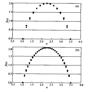
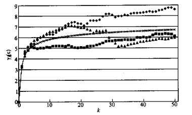
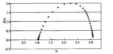
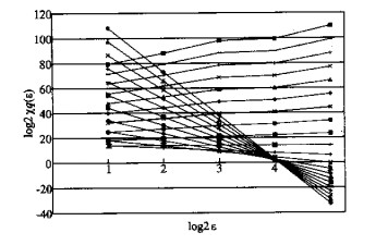
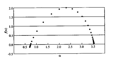
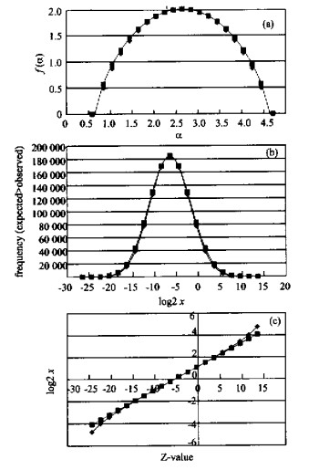
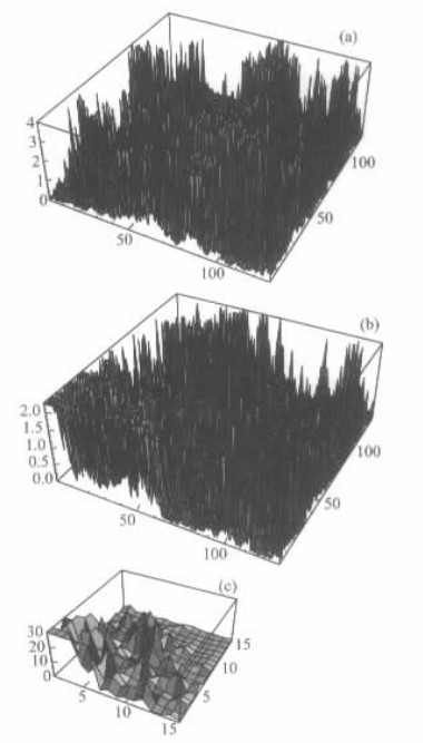
Using a simple multifractal model based on the model De Wijs, various geochemical map patterns for element concentration values are being simulated. Each pattern is self-similar on the average in that a similar pattern can be derived by application of the multiplicative cascade model used to any small subarea on the pattern. In other experiments, the original, self-similar pattern is distorted by superimposing a 2-dimensional trend pattern and by mixing it with a constant concentration value model. It is investigated how such distortions change the multifractal spectrum estimated by means of the 3-step method of moments. Discrete and continuous frequency distribution models are derived for patterns that satisfy the model of De Wijs. These simulated patterns satisfy a discrete frequency distribution model that as upper bound has a continuous frequency distribution to which it approaches in form when the subdivisions of the multiplicative cascade model are repeated indefinitely. This limiting distribution is lognormal in the center and has Pareto tails. Potentially, this approach has important implications in mineral and oil resource evaluation.