Figure
1.
Overall architecture of Inception-v3 (inferred from Szegedy et al., 2016).
| Citation: | Wei Lou, Dexian Zhang. Applications of Deep Learning in Mineral Discrimination: A Case Study of Quartz, Biotite and K-Feldspar from Granite. Journal of Earth Science, 2025, 36(1): 29-45. doi: 10.1007/s12583-022-1672-7

|
Mineral identification and discrimination play a significant role in geological study. Intelligent mineral discrimination based on deep learning has the advantages of automation, low cost, less time consuming and low error rate. In this article, characteristics of quartz, biotite and K-feldspar from granite thin sections under cross-polarized light were studied for mineral images intelligent classification by Inception-v3 deep learning convolutional neural network (CNN), and transfer learning method. Dynamic images from multi-angles were employed to enhance the accuracy and reproducibility in the process of mineral discrimination. Test results show that the average discrimination accuracies of quartz, biotite and K-feldspar are 100.00%, 96.88% and 90.63%. Results of this study prove the feasibility and reliability of the application of convolution neural network in mineral images classification. This study could have a significant impact in explorations of complicated mineral intelligent discrimination using deep learning methods and it will provide a new perspective for the development of more professional and practical mineral intelligent discrimination tools.
Rocks (ores) identification refers to the identifying of the mineral composition, mineral formation sequence, texture, structure and the own type of rocks (ores) (Liao, 2018), and is useful for tracing diagenesis and mineralization processes. During the works of rocks (ores) identification, mineral discrimination is vitally important for it provides the basic mineral information for the implementation and application of rock (ores) identification. Traditional mineral discrimination methods, from hand specimen identification, microscope observation, to microbeam analysis technology are facing problems such as high professional knowledge requirements, time-consuming, and costing (Lou et al., 2020).
In recent years, great breakthroughs have been made in the field of artificial intelligence, making the efficient intelligent discrimination of mineral a new possibility. Machine learning is one of the fastest developing fields of artificial intelligence. In the past two decades, common machine learning algorithms such as support vector machine (SVM) (Suykens and Vandewalle, 1999), K-nearest neighbor (KNN) (Cover and Hart, 1967), multinomial logistic regression (MLR) (Böhning, 1992), decision tree (DT) (Quinlan, 1986) have been widely applied to geological studies and achieved good performances (Itano et al., 2020; Hrstka et al., 2018; Ueki et al., 2018; Mollajan et al., 2016; Liu et al., 2008).
Deep learning is proposed by Hinton and Salakhutdinov (2006) on the basis of machine learning. It uses more layers of neural network to simulate human behavior to learn, and ensure learning ability by emphasizing the depth of network. With the development of technology, neural network starts from the multilayer perception (MLP) (Zhang et al., 2021), comes to artificial neural network (ANN) (Thompson et al., 2001), convolutional neural network (CNN) (LeCun et al., 1989), recurrent neural network (RNN) (Auli et al., 2013), deep belief neural networks (DBN) (Hinton et al., 2006), and generative adversarial networks (GAN) (Goodfellow et al., 2020). It is noteworthy that convolutional neural network has become one of the best algorithms to complete all kinds of image processing tasks whereby its virtue of weight sharing and local link (Lou et al., 2020; Zangeneh et al., 2020; Mohamed et al., 2018).
The development of convolutional neural network has experienced from network with few layers such as LeNet (LeCun et al., 1998) and AlexNet (Krizhevsky et al., 2017) to deep network such as VGGNet (Simonyan and Zisserman, 2014), SegNet (Badrinarayanan et al., 2017) and GoogleNet (Szegedy et al., 2015), and finally networks which have been improved the connection structure like ResNet (He et al., 2016) and DenseNet (Huang et al., 2017). At present, a large number of studies have been devoted to the application of advanced convolutional neural network in the extraction rocks (ores) and mineral images information (Guo et al., 2020; Xu and Zhou, 2018; Cheng et al., 2017; Aprile et al., 2014; Singh et al., 2010; Marmo et al., 2005; Thompson et al., 2001).
Opaque minerals in the ores are relatively stable in nature and less altered, they are smoothly studied by intelligent discrimination (Zhao et al., 2020; Li et al., 2020; Peng et al., 2019; Xu and Zhou, 2018). However, intelligent discrimination of transparent minerals in rocks are more difficult than those opaque minerals in ores (Guo et al., 2020; Iyas et al., 2020; Jiang et al., 2020; Ye et al., 2011; Baykan and Yılmaz, 2010; Thompson et al., 2001). In discrimination works about transparent minerals, intelligent mineral discrimination represented by sedimentary rock is more abundant, and the discrimination of minerals in igneous rock and metamorphic rock is less studied. Due to the complexity of minerals in metamorphic rock, intelligent mineral discrimination has not made a significant breakthrough in metamorphic rock so far. Therefore, this study focuses on mineral discrimination in igneous rock. Granite is a typical kind of igneous rock, it often forms huge rock mass and abundant of quartz, biotite and K-feldspar. These kinds of minerals are widely distributed in most of rocks and they are well-studied by geologists and mineralogists, which is suitable for the preliminary exploration of mineral intelligent discrimination.
Literature shows that convolution neural networks play an important role in mineral images intelligent classification in recent years (Guo et al., 2020; Li et al., 2020; Iyas et al., 2020; Jiang et al., 2020; Peng et al., 2019; Xu and Zhou, 2018), which proves that convolution neural network has the ability to extract patterned features of minerals after learning a large number of mineral images. However, most of the intelligent mineral discrimination works in the past decays was focused on the mineral characteristics under plane-polarized light, and few studies on that under cross-polarized light (Guo et al., 2020; Iyas et al., 2020; Jiang et al., 2020; Li et al., 2020; Zhao et al., 2020; Peng et al., 2019; Xu and Zhou, 2018; Ye et al., 2011; Baykan and Yılmaz, 2010; Thompson et al., 2001). Although the color, protrusions, cleavage and reflection color of minerals under plane-polarized light are very important, the interference color, extinction, homogeneity and internal reflection color of minerals under cross-polarized light are also worthy of attention. In this article, quartz, biotite and K-feldspar from granite thin sections under cross-polarized light were studied for minerals intelligent discrimination by deep learning methods. Consideration of the unique optical characteristics of these minerals under cross-polarized light will enhance the accuracy and reproducibility in the process of mineral discrimination. As a meaningful attempt of deep learning method in mineral images classification, this study could inspire more complicated minerals intelligent discrimination works in the future, and it will provide a new perspective for the development of more professional and practical mineral intelligent discrimination tools: For example, the development of mobile mineral discrimination software integrated with mineral optical libraries, which can not only assist professional geologists to discriminate minerals in real time in the field works, but also help non-professionals to study minerals more conveniently.
Classical convolutional neural networks include LeNet (LeCun et al., 1998), AlexNet (Krizhevsky et al., 2017), VGGNet (Simonyan and Zisserman, 2014), SegNet (Badrinarayanan et al., 2017), GoogleNet (Szegedy et al., 2015), and networks with improved connection structure like ResNet (He et al., 2016) and DenseNet (Huang et al., 2017). The appearance of LeNet lays the foundation of convolutional neural network. Its classic LeNet-5 contains three convolution layers and two full connection layers, which can input 32 × 32 gray image to achieve high accuracy handwritten numeral classification. AlexNet has five convolution layers and three fully connected layers, and it can be used for large size image (such as 224 × 224) classification. Then, GoogleNet deepens the depth and width of convolutional neural network. It uses convolution kernels of different sizes to form Inception modules, and stacks multiple Inception modules together to build a series of deep networks (Szegedy et al., 2017, 2016, 2015; Ioffe and Szegedy, 2015). Unlike GoogleNet, VGGNet uses convolution kernels of the same size, which proves the importance of depth to convolution neural network with a simpler topology. ResNet and DenseNet are committed to changing the connection structure of CNN: ResNet uses the shortcut branch in residual block to make some network layers obtain additional output of the former layer as input, which speeds up the network training. And DenseNet uses a more aggressive dense connection structure named dense block, to make each layer accept the output of all previous layers as its additional input, which further improves the network performance.
With the continuous improvement of CNNs, the classification performance of these above advanced CNNs all can meet the needs of general classification tasks well. When further considering the computational cost of networks, Inception-v3 (Szegedy et al., 2016) of GooleNets was used as our pretraining model. The original training dataset of the Inception-v3 contains 1.2 million images of 1 000 categories. It has been trained on a computer equipped with 8 Tesla K40 GPUs for several weeks and contains about 25 million parameters (Zhang et al., 2018). Compared with other deep networks such as VGGNet and ResNet, the parameters of Inception-v3 are greatly reduced. Therefore, it can be used for training and testing in the environment of limited computing memory (such as a computer equipped with a common GPU) (Zhang et al., 2018; Szegedy et al., 2016). Moreover, Literatures also show that Inception-v3 has a good performance for mineral discrimination (Li et al., 2020; Peng et al., 2019; Bai et al., 2018; Zhang et al., 2018).
In 2015, Google proposed the original GoogleNet (Szegedy et al., 2015). Because of the innovative use of inception module in GoogleNet, it is also known as Inception-v1. In the following two years, GoogleNet has been continuously improved by its team, and the Inception module has been inherited. As a result, Inception-v2 (Ioffe and Szegedy, 2015), Inception-v3 (Szegedy et al., 2016), and Inception-v4 (Szegedy et al., 2017) have appeared successively.
The Inception-v1 uses different size convolutional kernels in parallel to form the concept module, which have the ability to obtain image features from different scales, and greatly improves the performance of the network. Based on the Inception-v1, the Inception-v2 introduces batch normalization (BN) (Ioffe and Szegedy, 2015), which solves the gradient disappearance in training and accelerates the network training. Next, the Inception-v3 (Szegedy et al., 2016) has made more improvements based on Inception-v2, mainly as follows: ① Convolution decomposition is introduced. ② A more effective method of feature map size reduction is applied. ③ Label smoothing regulation (LSR) is proposed to regularize the network output and suppress the overconfidence prediction of the network. The latest Inception-v4 mainly realizes the combination of GoogleNets and ResNet, proposing a rich variety of concept Inception-ResNet (Szegedy et al., 2017).
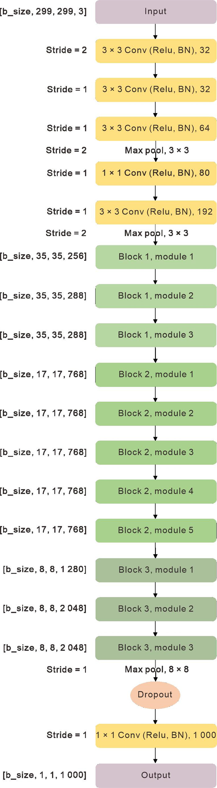
Inception-v3 is the best work of GoogleNets which can fully reflect their design concepts. It not only has strong feature extraction and classification ability, but also has the characteristics of low cost and strong portability, which can be used well in the experimental environment with limited computing ability. Inferred from the source code of Inception-v3 (Szegedy et al., 2016), the overall structure of the network is shown in Figure 1. The Inception-v3 includes three module blocks, and each block includes 3, 5 and 3 inception modules respectively. All of these modules strictly obey the design rules of Inception-v3 mentioned in the previous paragraph. Because of the implementation of these new design concepts, Inception-v3 has become one of the most praised representative products of convolutional neural network.
Transfer learning refers to using knowledge learned from previous tasks to complete new learning tasks (Liu et al., 2018; Pan and Yang, 2010). Most traditional machine learning methods are based on an assumption that training samples and test samples should come from similar space and have similar distribution (Xie, 2016). However, in many practical applications, this assumption is difficult to satisfied (Dai et al., 2007). Therefore, traditional machine learning needs to recollect training samples for different learning tasks and build models from scratch, which is bound to waste a lot of time (Zhang et al., 2018).
Transfer learning method breaks the above limitation. It does not require that samples in different learning tasks should keep the same distribution. As long as there is a certain correlation between two learning tasks, the model trained on the source learning task can be used to training and testing on the target learning task (Wang, 2017). Transfer learning migrates the knowledge learned from similar fields (Patel et al., 2015), making the traditional learning from scratch into cumulative learning. It not only reduces the cost of model training, but also significantly improves the performance of model learning (Pan and Yang, 2010).
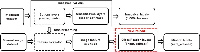
For the use of pretraining model in transfer learning, there are mainly two methods: finetune and feature extraction. Taking the deep learning network model as an example, finetune uses the target learning task data to retrain all layers of the pretrained network. And feature extraction keeps all the parameters of the bottom layers of the pretrained network unchanged, reconstructs and retrains the last output layer of the network. Because the training workload and computing memory required in finetune are relatively high, feature extraction becomes the first choice of transfer learning when computing condition become an important factor to be considered. The Inception-v3 mentioned in 1.2 was pretrained on ImageNet dataset (contains 1.2 million images of 1 000 categories), which has the ability to extract effective features from images. Although the source learning task data of Inception-v3 CNN and our mineral images data for mineral discrimination come from different spaces, these two tasks are both essentially about images classification. Therefore, Inception-v3 CNN was selected as the feature extractor to carry out the study of mineral discrimination based on transfer learning in this article.
Figure 2 shows the workflow of transfer learning using Inception-v3 CNN. The "softmax" function used in classification layer (Zheng et al., 2019; LeCun et al., 2015) is an activation function. It is often used for multi-classifications by mapping the scores of the output layer to (0, 1) in the form of probability. Considering that the number of categories corresponding to the source classification task of the Inception-v3 is 1 000, while the number of categories corresponding to our target task is 3 (quartz, biotite and K-feldspar), the output layer of the backbone and auxiliary classifier of the Inception-v3 have been rebuilt.
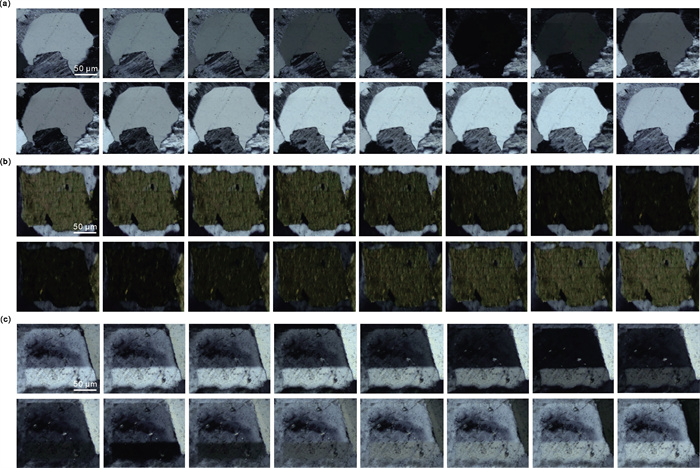
A polarizing microscope was employed to collect the image data of granite thin sections at 16 angles from 0° to 90° with equal interval under cross-polarized light. Thirty mineral particles from each type of mineral: quartz, biotite and K-feldspar in granite thin sections were selected and their images were used to establish our mineral images dataset (the dataset contains 90 × 16 = 1 440 images). Figure 3 shows some image data in the mineral dataset. Next, these images were randomly divided into training set (1 170 pictures) and validation set (270 pictures) according to the ratio of 8 : 2 for the training and validation of Inception-v3 CNN in the process of transfer learning. Figure 4 shows the process of image data division taking a single mineral particle as an example. All 90 mineral particles in our whole dataset are divided in the same way.
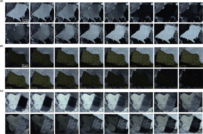

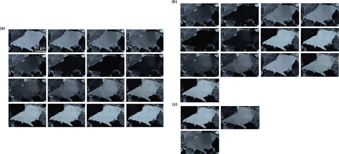
In the test period, we select two additional mineral particles for quartz, biotite and K-feldspar respectively, and input 16 pictures of each mineral particle into the trained Inception-v3 CNN to observe the mineral images classification output. Our test dataset totally has 6 × 16 = 96 pictures, Figure 5 shows part of the picture data of the test dataset.

When using optical microscope for data acquisition, and uniform parameters should be set to obtain image data with consistent color intensity, light intensity and white balance information. In addition, in order to facilitate the training of the network model, the collected images involved in this study need to be preprocessed.
(1) Image labeling. The particle images of each mineral category were selected by professionals under the microscope and labeled by the category of the main mineral in the middle of the image. Then the category name of mineral images will be automatically converted into digital labels by algorithm. Specifically, each mineral category corresponding to a unique digital label. In this article, the digital label for mineral category of biotite, quartz and K-feldspar is 0, 1 and 2, respectively. In this way, categories of mineral were represented by unique digital labels for better processed by computer. During the training process, the network model will be continuously optimized by minimizing the loss function between the predicted labels and the true labels of the input images (Hinton et al., 2012).
(2) Data augmentation. Data augmentation can effectively reduce over fitting and optimize the training effect of the network model (Smirnov et al., 2014). In this study, collected image data are randomly cropped and randomly flipped horizontally following the way of (Krizhevsky et al., 2017). Figure 6 shows the schematic diagram of image cropping and horizontal flipping. Because the input image size of Inception-v3 CNN is 229 × 229, the side lengths of the original image are constrained roughly in the range of [229, 382] (the side lengths of the cropped image are more than 3/5 of that of the original image), and the main category mineral of original image is selected for occupying most of the image area. In this way, the categories of main minerals are still retained in all cropped images.

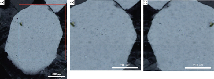
(3) Image standardization. Image standardization enables the computer to better learn the distribution of images pixel value, speeding up the calculation of model. Figure 7 shows the image before and after standardization. For an image dataset, the process of image standardization is as follows.
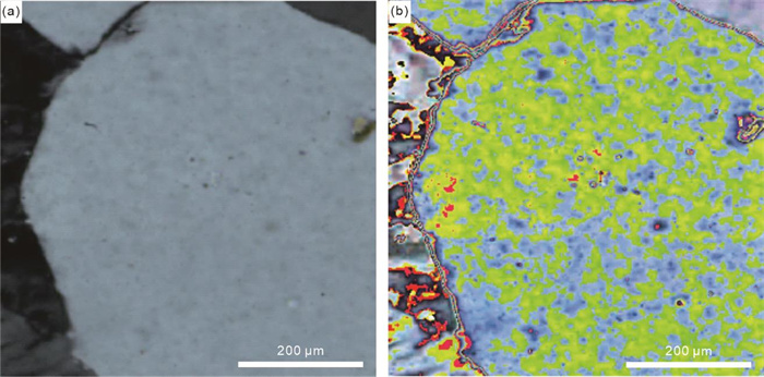
Step 1: Calculating the mean (recorded as Meani) and standard deviation (recorded as Stdi) of all images in the whole dataset on each channel i (gray image i = 1, RGB image i = 3).
Step 2: For all channels in a picture, subtracting the channel's mean value (recorded as Meani) of the dataset from the pixel value on the corresponding channel of the picture, and then divide it by the channel's standard deviation (recorded as Stdi). both the Meani and Stdi are got in the step1.
|
Imagestd=Imagei−MeaniStdi(i=1,2,3) |
(1) |
"Image" is a three-dimensional tensor of the input image, the shape of the tensor corresponding to the size of image's height, width and channels. For RBG image the channels = 3. The subscript i denotes the ith channels of the image. And $ "Mea{n}_{i} $", $ "St{d}_{i}" $ are the mean value, standard deviation value in ith channels of whole image dataset.
During the experiment, the Inception-v3 CNN was employed for transfer learning. The specific experiment details are as follows.
The optimizer used in training network was Adam (adaptive motion estimation) (Kingma and Ba, 2014) and loss function was cross entropy loss. cross entropy loss is particularly useful when training a classification problem with muti-classes, and it describes the distance between the probability distribution of the predicted value and the ground truth, so it usually appears together with "softmax" function (mentioned in 1.3). For "N" input samples, total cross entropy loss between their predicted values and the ground truths is present in Formula (2). Then their average cross entropy loss is present in Formula (3).
|
Loss(y',y)=−∑Ni=1y'ilog(yi) |
(2) |
|
AvgLoss(y',y)=1NLoss(y',y) |
(3) |
For "N" input samples, "i" is the ith sample. "yi'" is the predicted value of the input sample i, and yi is the ground truth of the input sample i.
For most applications, small batch gradient descent is the recommended variant of gradient descent, especially in deep learning. "Batch size" is usually adjusted to suitable for the memory requirements of GPU or CPU hardware, such as 32, 64, 128, 256, etc. On our mineral image dataset with relatively limited samples, Inception-v3 CNN was trained preferably using batch size 32 for 10 epochs (selection of batch size see Figures S1, S2, S3 in supplementary information). The initial learning rate was set to 0.002, and learning rate decay would not be carried out because this initial learning rate was small enough. The setting of other network parameters is consistent with that of original Inception-v3.
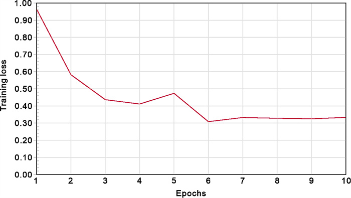
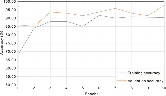
The change of the loss function value of the network during the training process is plotted in Figure 8, and the accuracy of the network on training set and validation set are shown in Figure 9. It can be clearly seen in Figure 8 that with the increase of network training epoch, the loss function value of network continues to decrease, showing the improvement classification ability of our network. In early four epochs, the loss function decreases sharply, and then and the downward trend begins to slow down. The network almost reaches convergence after the sixth epoch marked by the stability of the loss curve, which means our network has a fast convergence speed. The loss value of the network after convergence is about 0.32. In Figure 9, the bule line represents the accuracy of the network on the training set with the change of training times, and the orange line represents the accuracy of the network on the validation set after each training. The accuracy of the validation set should be higher than that of the training set (consistent with Figure 9), because the prediction on the validation set is carried out after the model be trained and optimized in each epoch. The accuracy curve on the training set shows that with the convergence of the model training (about in the sixth epoch), the accuracy of the model on the training set reaches the highest value about 91.00%, and then tends to be stable. This is consistent with the training loss function in Figure 8. In the validation set, the model achieves a high accuracy at seventh epoch, which is about 95.00%. In the following two epochs, the validation accuracy reduces in a small range, which may be caused by overfitting (Smirnov et al., 2014). In the end of the tenth epoch, the final accuracy of the model on the validation set reaches 97.00%.

In order to test the reliable mineral discrimination ability of the trained Inception-v3, images not included in the mineral dataset described in Section 2.1 were selected for testing. Two extra mineral particles for quartz, biotite and K-feldspar respectively were involved in our test phase. Each particle contains 16 mineral images described in Section 2.1. The 6 × 16 = 96 test images were input into Inception-v3 CNN for classification, and details of classification results are listed in Table 1.
| True label | Samples | Picture numbers | Predicted label | Prediction probability | Accuracy | Samples | Picture numbers | Predicted label | Prediction probability | Accuracy |
| Quartz | Sample 1 | 1 | Quartz | 0.999 | 100.00% | Sample 2 | 1 | Quartz | 0.956 | 100.00% |
| 2 | Quartz | 0.999 | 2 | Quartz | 0.938 | |||||
| 3 | Quartz | 1.000 | 3 | Quartz | 0.725 | |||||
| 4 | Quartz | 0.982 | 4 | Quartz | 0.936 | |||||
| 5 | Quartz | 0.969 | 5 | Quartz | 0.968 | |||||
| 6 | Quartz | 0.902 | 6 | Quartz | 0.994 | |||||
| 7 | Quartz | 0.997 | 7 | Quartz | 0.991 | |||||
| 8 | Quartz | 0.998 | 8 | Quartz | 0.928 | |||||
| 9 | Quartz | 0.996 | 9 | Quartz | 0.959 | |||||
| 10 | Quartz | 0.999 | 10 | Quartz | 0.839 | |||||
| 11 | Quartz | 0.934 | 11 | Quartz | 0.963 | |||||
| 12 | Quartz | 0.983 | 12 | Quartz | 0.877 | |||||
| 13 | Quartz | 0.979 | 13 | Quartz | 0.758 | |||||
| 14 | Quartz | 0.984 | 14 | Quartz | 0.977 | |||||
| 15 | Quartz | 0.978 | 15 | Quartz | 0.858 | |||||
| 16 | Quartz | 0.998 | 16 | Quartz | 0.941 | |||||
| Biotite | Sample 1 | 1 | Biotite | 0.991 | 100.00% | Sample 2 | 1 | Biotite | 0.812 | 93.75% |
| 2 | Biotite | 0.919 | 2 | K-feldspar | 0.581 | |||||
| 3 | Biotite | 0.999 | 3 | Biotite | 0.887 | |||||
| 4 | Biotite | 0.981 | 4 | Biotite | 0.818 | |||||
| 5 | Biotite | 0.946 | 5 | Biotite | 0.984 | |||||
| 6 | Biotite | 0.998 | 6 | Biotite | 0.955 | |||||
| 7 | Biotite | 0.991 | 7 | Biotite | 0.994 | |||||
| 8 | Biotite | 0.997 | 8 | Biotite | 0.932 | |||||
| 9 | Biotite | 0.997 | 9 | Biotite | 0.932 | |||||
| 10 | Biotite | 0.936 | 10 | Biotite | 0.809 | |||||
| 11 | Biotite | 0.988 | 11 | Biotite | 0.966 | |||||
| 12 | Biotite | 0.997 | 12 | Biotite | 0.980 | |||||
| 13 | Biotite | 0.995 | 13 | Biotite | 0.912 | |||||
| 14 | Biotite | 0.920 | 14 | Biotite | 0.807 | |||||
| 15 | Biotite | 0.760 | 15 | Biotite | 0.996 | |||||
| 16 | Biotite | 0.930 | 16 | Biotite | 0.787 | |||||
| 1 | K-feldspar | 0.975 | 1 | K-feldspar | 0.961 | 87.50% | ||||
| 2 | K-feldspar | 0.947 | 2 | K-feldspar | 0.976 | |||||
| 3 | K-feldspar | 0.955 | 3 | K-feldspar | 0.971 | |||||
| 4 | K-feldspar | 0.749 | 4 | K-feldspar | 0.603 | |||||
| 5 | K-feldspar | 0.965 | 5 | K-feldspar | 0.982 | |||||
| 6 | K-feldspar | 0.927 | 6 | K-feldspar | 0.951 | |||||
| 7 | K-feldspar | 0.975 | 7 | K-feldspar | 0.977 | |||||
| 8 | K-feldspar | 0.977 | 8 | K-feldspar | 0.884 | |||||
| 9 | K-feldspar | 0.830 | 9 | K-feldspar | 0.579 | |||||
| 10 | K-feldspar | 0.954 | 10 | Biotite | 0.503 | |||||
| 11 | K-feldspar | 0.987 | 11 | K-feldspar | 0.875 | |||||
| 12 | K-feldspar | 0.824 | 12 | K-feldspar | 0.806 | |||||
| 13 | K-feldspar | 0.975 | 13 | K-feldspar | 0.967 | |||||
| 14 | K-feldspar | 0.907 | 14 | K-feldspar | 0.564 | |||||
| 15 | K-feldspar | 0.519 | 15 | K-feldspar | 0.707 | |||||
| 16 | Quartz | 0.537 | 16 | Biotite | 0.556 | |||||
| The bold marks indicate wrong classification of mode. | ||||||||||
 DownLoad:
CSV
DownLoad:
CSV
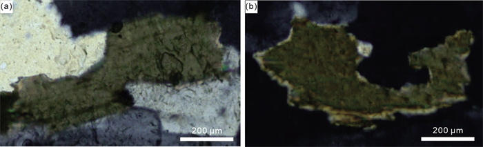
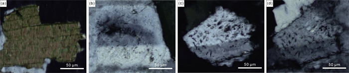
Table 1 shows that most of the images in all mineral particles are classified correctly, and there are only four images with wrong classification. These misclassified images are retrieved from dataset and shown in Figure 10 for further discussion. The poor-quality samples that may causing biotite images classification errors are also shown in Figure 11, we will give our explanation in the discussion section later.

From Table 1, it can be clearly seen that all the pictures of the two mineral particles of quartz are classified correctly, and the classification accuracy of quart images is 100.00%. In particular, all the 16 images of No. 1 quartz sample are classified into the correct category with a high prediction probability of more than 0.900. In No. 1 quartz sample, the highest prediction probability is 1.000 in No. 3 image, the lowest prediction probability is 0.902 in No. 6 image, and the average prediction probability of all images is 0.981. In No. 2 quartz sample, the highest prediction probability is 0.994 of No.6 image, the lowest prediction probability is 0.725 of No.3 image, and the average prediction probability of all images is 0.913.
All these 16 images of No. 1 biotite sample are classified correctly, and the classification accuracy is 100.00%. Among them, the highest prediction probability in picture 3 is 0.999, the lowest prediction probability in picture 15 is 0.760, and the average prediction probability in all pictures is 0.959. In No. 2 biotite sample, No. 2 image is misclassified as K-feldspar, and the classification accuracy is 93.75%. The highest prediction probability is 0.996 in picture 15, and the lowest prediction probability is 0.581 in picture 2. The average prediction probability of all images with correct classification is 0.905.
In No. 1 K-feldspar sample, there is one picture wrongly classified (picture 16 is misclassified as quartz), and the classification accuracy is 93.75%. Among them, the highest prediction probability is 0.987 of picture 11, the lowest prediction probability is 0.519 of picture 15, the prediction probability of picture 16 with wrong classification is 0.537, and the average prediction probability of all pictures with correct classification is 0.898. In No. 2 K-feldspar sample, there are two mineral images classified incorrectly (No.10 and No.16 images are misclassified as biotite), and the classification accuracy is 87.50%. Among them, the highest prediction probability is 0.982 for picture 5, the lowest prediction probability is 0.503 for picture 10. As for picture 16, the prediction probability is 0.556. The average prediction probability for all correctly classified images is 0.843, while the average prediction probability for the two wrongly classified images is 0.530.
The average discrimination accuracy of quartz, biotite and K-feldspar were summarized in Table 2. The discrimination accuracy of quartz is the highest, and the average discrimination accuracy is 100.00%. The average discrimination accuracy of biotite and K-feldspar is 96.88% and 90.63% respectively. The discrimination accuracy of all mineral categories is above 90.00%, which indicates that our transfer learning method based on Inception-v3 CNN has good performance on mineral images classification collected from different angles under cross-polarized light.
| Mineral category | Samples | Correct number/total | Accuracy | Average accuracy |
| Quartz | Sample 1 | 16/16 | 100.00% | 100.00% |
| Sample 2 | 16/16 | 100.00% | ||
| Biotite | Sample 1 | 16/16 | 100.00% | 96.88% |
| Sample 2 | 15/16 | 93.75% | ||
| K-feldspar | Sample 1 | 15/16 | 93.75% | 90.63% |
| Sample 2 | 14/16 | 87.50% |
DownLoad:
CSV
It can be seen from Table 1 that the Inceptopn-v3 transfer learning model can successfully classify most of the mineral images into the correct categories, which strongly indicates this model is very competent in mineral images classification task. Furthermore, a large part of the correctly classified images can obtain more than 0.900 prediction probability, while the images with wrong classification usually with low prediction probability (about 0.500). This shows that the model is confident in the mineral image features it learns. That is, when model recognizes the features of an input mineral image as known-features, it can immediately identify the mineral category it belongs to. However, one observed limitation of this network model is when the input image's feature is not good agree with the features learned by the model, the model still classify the image into a category with a relative high prediction score compulsorily.
The average discrimination accuracies of quartz, biotite and K-feldspar in Table 2 are all more than 90.00%, which is higher than the general level of mineral discrimination accuracies obtained in related studies (Guo et al., 2020; Iyas et al., 2020; Li et al., 2020; Zhao et al., 2020; Peng et al., 2019; Xu and Zhou, 2018; Ye et al., 2011; Baykan and Yılmaz, 2010; Thompson et al., 2001). The Inception-v3 transfer learning model has achieved perfect performance in quartz images classification, and the classification accuracy is 100.00%. Quartz is a rock forming mineral with the strongest weathering stability, and under cross-polarized light it has a wavy extinction that can be distinguished from other minerals (Iyas et al., 2020). Besides, the quartz samples in our granite thin sections are especially typical: the particle's surface is smooth, the interference color is of high grade of purity, and the edge of mineral particles is clear, which is easy to be learned by the model. Classification of quartz image in other related studies have also achieved good results, and the classification accuracies are in the range of 85.00%–100.00% (Guo et al., 2020; Peng et al., 2019; Ye et al., 2011; Baykan and Yılmaz, 2010; Thompson et al., 2001). In our study, the classification accuracy of quartz images can be stably close to 100.00%.
For further understanding of the misclassification situation of the Inception-v3 transfer learning model, the confusion matrix of the model test results is shown in Table 3. The numerical value in Table 3 represents the probability that the model classifies an actual mineral image into a prediction category.
| Mineral category | Quartz | Biotite | K-feldspar |
| Quartz | 100.00% | 0 | 0 |
| Biotite | 0 | 96.88% | 3.12% |
| K-feldspar | 3.12% | 6.25% | 90.63% |
DownLoad:
CSV
In our case of misclassification, K-feldspar images have the highest error rate. On the one hand, the K-feldspar series includes orthoclase, microcline, sanidine according to the tiny difference of mineral texture, but the number of K-feldspar samples in this study is only 30, which is too less for the model to acquire all the knowledge of K-feldspar categories. Mineral discrimination errors caused by micro texture differences or micro compositional change are also confirmed by Thompson et al. (2001) and Peng et al. (2019). Thompson et al. (2001) also emphasized the importance of texture features in improving the accuracy of mineral discrimination. On the other hand, the weathering stability of K-feldspar is worse than that of quartz, and it is prone to alteration (Zhai et al., 2020). In our granite thin section, the K-feldspar particles have varying degrees of alteration, most of which formed mica minerals after alteration, which led to the poor optical characteristics under cross-polarized light. In addition, there are some interferences with similar image characteristics. For example, No. 16 picture of No. 1 K-feldspar sample (Figure 10b) is misclassified as quartz. The reason is that a large number of first-order gray samples with similar interference color of No. 16 picture of No. 1 K-feldspar sample in quartz image library were selected. Due to quartz, and K-feldspar have more or less the same interference color, this wrong discrimination phenomenon also appears in (Guo et al., 2020; Iyas et al., 2020; Thompson et al., 2001). Mineral discrimination performance of network is closely related to the quantity and quality of training data. The training data should fully reflect the characteristics of the object to be studied. Therefore, it is suggested to use reasonable large-scale training dataset with good quality to train the network (Thompson et al., 2001), especially for K-feldspar and other minerals with great diversity.
A misclassification case occurred in the biotite images. After analysis, the shape of some sample particles in the biotite dataset is too narrow and long (Figure 11a), which leads to the image area occupied by the main minerals insufficient. This defect may be further magnified in the image cropping process, thus affecting the training and testing of the model. In order to avoid the interference of clipping, the main minerals of an image should occupy most of the image area (Guo et al., 2020). Some particles in biotite dataset have reaction rim texture (Figure 11b) (Wang et al., 2015), which affect the test results too.
From the above examples, it can be seen that although the discrimination behavior of convolutional neural network is a black box operation that cannot be explained in theory, its internal logical relationship and reasonable results explanations can still be given through the analysis of discrimination cases. Some inspiration for improving model accuracy can also be found at the same time.
In the works of mineral discrimination, the mineral images classification under cross-polarized light needs more training data than that under plane-polarized light, which resulting in less studies. However, for some transparent minerals such as quartz and feldspar, their optical characteristics under cross-polarized light are more distinctive, and the discrimination performance can be significantly improved by using their images under cross-polarized light (Iyas et al., 2020; Thompson et al., 2001). This is strongly confirmed by the high classification accuracy of quartz and K-feldspar images under cross-polarized in our study. Therefore, the implementation of mineral images classification under cross-polarized light plays an important role in improving the accuracy of mineral discrimination.
Due to the limited time and experimental conditions, the mineral optical dataset established in this study is relatively simple, and the quality of rock thin sections in our experiment is not quite satisfied. This study only studies the common minerals of acid rock (granite) in igneous rocks. Typical minerals of other intermediate rock, mafic rock and ultramafic rock will be integrated in the following studies.
Three kinds of common minerals in granite: quartz, biotite and K-feldspar under cross-polarized light were studied for mineral images intelligent classification by Inception-v3 CNN and transfer learning method. The accuracy of quartz, biotite and K-feldspar is 100.00%, 96.88% and 90.63% respectively. Our network can classify most of the test images into the correct category with prediction probability of more than 0.900.
It is not our ultimate aim to study the discrimination of these three common and well-known minerals in granite, but to discuss the feasibility of convolution neural network in mineral intelligence discrimination. This study represents a step forward compared to previous studies by bringing the mineral images intelligent classification from static images classification to dynamic multi-angles images classification. And it could provide a new perspective for the development of more professional and practical mineral intelligent discrimination applications.
ACKNOWLEDGMENTS: This research was funded by the National Natural Science Foundation of China (Nos. 41672082, 42030809). The authors sincerely thank Zhiyi Liu and Lu Luo from Zeiss China for theirs great assistance in thin section scanning. Two anonymous reviewers are appreciated for their constructive suggestion to enhance this article. The final publication is available at Springer via https://doi.org/10.1007/s12583-022-1672-7.| Aprile, A., Castellano, G., Eramo, G., 2014. Combining Image Analysis and Modular Neural Networks for Classification of Mineral Inclusions and Pores in Archaeological Potsherds. Journal of Archaeological Science, 50: 262–272. https://doi.org/10.1016/j.jas.2014.07.017 |
| Auli, M., Galley, M., Quirk, C., et al., 2013. Joint Language and Translation Modeling with Recurrent Neural Networks. Proceedings of the 2013 Conference on Empirical Methods in Natural Language Processing (EMNLP), Oct. 18–21, 2013, Seattle. 1044–1054 |
| Badrinarayanan, V., Kendall, A., Cipolla, R., 2017. SegNet: A Deep Convolutional Encoder-Decoder Architecture for Image Segmentation. IEEE Transactions on Pattern Analysis and Machine Intelligence, 39(12): 2481–2495. https://doi.org/10.1109/TPAMI.2016.2644615 |
| Bai, L., Yao, Y., Li, S. T., et al., 2018. Mineral Compositionanalysis of Rock Image Based on Deep Learning Feature Extraction. China Mining Magazine, 27(7): 178–182 (in Chinese with English Abstract) |
| Baykan, N. A., Yılmaz, N., 2010. Mineral Identification Using Color Spaces and Artificial Neural Networks. Computers & Geosciences, 36(1): 91–97. https://doi.org/10.1016/j.cageo.2009.04.009 |
| Böhning, D., 1992. Multinomial Logistic Regression Algorithm. Annals of the Institute of Statistical Mathematics, 44(1): 197–200. https://doi.org/10.1007/bf00048682 |
| Cheng, G. J., Guo, W. H., Fan, P. Z., 2017. Study on Rock Image Classification Based on Convolution Neural Network. Journal of Xi'an Shiyou University (Natural Science Edition), 32(4): 116–122. https://doi.org/10.3969/j.issn.1673-064X.2017.04.020 (in Chinese with English Abstract) |
| Cover, T., Hart, P., 1967. Nearest Neighbor Pattern Classification. IEEE Transactions on Information Theory, 13(1): 21–27. https://doi.org/10.1109/TIT.1967.1053964 |
|
Dai, W. Y., Yang, Q., Xue, G. R., et al., 2007. Boosting for transfer Learning. Proceedings of the 24th International Conference on Machine Learning, Jun. 20–24, 2007, Corvalis. 193–200. |
| Goodfellow, I., Pouget-Abadie, J., Mirza, M., et al., 2020. Generative Adversarial Networks. Communications of the ACM, 63(11): 139–144. https://doi.org/10.1145/3422622 |
| Guo, Y. J., Zhou, Z., Lin, H. X., et al., 2020. The Mineral Intelligence Identification Method Based on Deep Learning Algorithms. Earth Science Frontiers, 27(5): 39–47. https://doi.org/10.13745/j.esf.sf.2020.5.45 (in Chinese with English Abstract) |
|
He, K. M., Zhang, X. Y., Ren, S. Q., et al., 2016. Deep Residual Learning for Image Recognition. Proceedings of the 2016 IEEE Conference on Computer Vision and Pattern Recognition (CVPR), Jun. 27–30, 2016, Las Vegas. 770–778. |
| Hinton, G. E., Osindero, S., Teh, Y. W., 2006. A Fast Learning Algorithm for Deep Belief Nets. Neural Computation, 18(7): 1527–1554. https://doi.org/10.1162/neco.2006.18.7.1527 |
| Hinton, G. E., Salakhutdinov, R. R., 2006. Reducing the Dimensionality of Data with Neural Networks. Science, 313(5786): 504–507. https://doi.org/10.1126/science.1127647 |
| Hinton, G. E., Srivastava, N., Krizhevsky, A., et al., 2012. Improving Neural Networks by Preventing Co-Adaptation of Feature Detectors. arXiv: 1207.0580. http://arxiv.org/abs/1207.0580v1 |
| Hrstka, T., Gottlieb, P., Skála, R., et al., 2018. Automated Mineralogy and Petrology-Applications of TESCAN Integrated Mineral Analyzer (TIMA). Journal of Geosciences, 47–63. https://doi.org/10.3190/jgeosci.250 |
|
Huang, G., Liu, Z., Van Der Maaten, L., et al., 2017. Densely Connected Convolutional Networks. 2017 IEEE Conference on Computer Vision and Pattern Recognition (CVPR). Proceedings of the 2017 IEEE Conference on Computer Vision and Pattern Recognition (CVPR), Jul. 21–26, 2017, Honolulu. 2261–2269. |
|
Ioffe, S., Szegedy, C., 2015. Batch Normalization: Accelerating Deep Network Training by Reducing Internal Covariate Shift. Proceedings of the 32nd International Conference on International Conference on Machine Learning, Jul. 6–11, 2015, Lille. 448–456. |
| Itano, K., Ueki, K., Iizuka, T., et al., 2020. Geochemical Discrimination of Monazite Source Rock Based on Machine Learning Techniques and Multinomial Logistic Regression Analysis. Geosciences, 10(2): 63. https://doi.org/10.3390/geosciences10020063 |
| Iyas, M. R., Setiawan, N. I., Warmada, I. W., 2020. Mask R-CNN for Rock-Forming Minerals Identification on Petrography, Case Study at Monterado, West Kalimantan. E3S Web of Conferences, 200: 06007. https://doi.org/10.1051/e3sconf/202020006007 |
| Jiang, F., Li, N., Zhou, L. L., 2020. Grain Segmentation of Sandstone Images Based on Convolutional Neural Networks and Weighted Fuzzy Clustering. IET Image Processing, 14(14): 3499–3507. https://doi.org/10.1049/iet-ipr.2019.1761 |
| Kingma, D. P., Ba, J., Hammad, M. M., 2014. Adam: A Method for Stochastic Optimization. arXiv: 1412.6980. http://arxiv.org/abs/1412.6980v9 |
| Krizhevsky, A., Sutskever, I., Hinton, G. E., 2017. ImageNet Classification with Deep Convolutional Neural Networks. Communications of the ACM, 60(6): 84–90. https://doi.org/10.1145/3065386 |
| LeCun, Y., Bengio, Y., Hinton, G., 2015. Deep Learning. Nature, 521(7553): 436–444. https://doi.org/10.1038/nature14539 |
| LeCun, Y., Boser, B., Denker, J. S., et al., 1989. Backpropagation Applied to Handwritten Zip Code Recognition. Neural Computation, 1(4): 541–551. https://doi.org/10.1162/neco.1989.1.4.541 |
| LeCun, Y., Bottou, L., Bengio, Y., et al., 1998. Gradient-Based Learning Applied to Document Recognition. Proceedings of the IEEE, 86(11): 2278–2324. https://doi.org/10.1109/5.726791 |
| Li, M. C., Liu, C. Z., Zhang, Y., et al., 2020. A Deep Learning and Intelligent Recognition Method of Image Data for Rock Mineral and Its Implementation. Geotectonica et Metallogenia, 44(2): 203–211. https://doi.org/10.16539/j.ddgzyckx.2020.02.004 (in Chinese with English Abstract) |
| Liao, B. B., 2018. Analysis of Current Status and Development Trend of Rock and Mineral Identification. Resource Information and Engineering, 33(2): 27–28 (in Chinese with English Abstract) |
| Liu, X. P., Luan, X. D., Xie, Y. X., et al., 2018. Transfer Learning Research and Algorithm Review. Journal of Changsha University, 32(5): 28–31, 36. https://doi.org/10.3969/j.issn.1008-4681.2018.05.008 (in Chinese with English Abstract) |
| Liu, Y. B., Cao, S. G., Liu, Y. C., 2008. Discussion on Analytical Method for LS-SVM Based Mesoscopic Rock Images. Chinese Journal of Rock Mechanics and Engineering, 27(5): 1059–1065. https://doi.org/10.3321/j.issn:1000-6915.2008.05.023 (in Chinese with English Abstract) |
| Lou, W., Zhang, D. X., Bayless, R. C., 2020. Review of Mineral Recognition and Its Future. Applied Geochemistry, 122: 104727. https://doi.org/10.1016/j.apgeochem.2020.104727 |
| Marmo, R., Amodio, S., Tagliaferri, R., et al., 2005. Textural Identification of Carbonate Rocks by Image Processing and Neural Network: Methodology Proposal and Examples. Computers & Geosciences, 31(5): 649–659. https://doi.org/10.1016/j.cageo.2004.11.016 |
| Mohamed, A. A., Berg, W. A., Peng, H., et al., 2018. A Deep Learning Method for Classifying Mammographic Breast Density Categories. Medical Physics, 45(1): 314–321. https://doi.org/10.1002/mp.12683 |
| Mollajan, A., Ghiasi-Freez, J., Memarian, H., 2016. Improving Pore Type Identification from Thin Section Images Using an Integrated Fuzzy Fusion of Multiple Classifiers. Journal of Natural Gas Science and Engineering, 31: 396–404. https://doi.org/10.1016/j.jngse.2016.03.030 |
| Pan, S. J., Yang, Q., 2010. A Survey on Transfer Learning. IEEE Transactions on Knowledge and Data Engineering, 22(10): 1345–1359. https://doi.org/10.1109/TKDE.2009.191 |
| Patel, V. M., Gopalan, R., Li, R. N., et al., 2015. Visual Domain Adaptation: A Survey of Recent Advances. IEEE Signal Processing Magazine, 32(3): 53–69. https://doi.org/10.1109/MSP.2014.2347059 |
| Peng, W. H., Bai, L., Shang, S. W., et al., 2019. Common Mineral Intelligent Recognition Based on Improved InceptionV3. Geological Bulletin of China, 38(12): 2059–2066 (in Chinese with English Abstract) |
| Quinlan, J. R., 1986. Induction of Decision Trees. Machine Learning, 1(1): 81–106. https://doi.org/10.1007/BF00116251 |
|
Simonyan, K., Zisserman, A., 2014. Very Deep Convolutional Networks for Large-Scale Image Recognition. arXiv: 1409.1556. |
| Singh, N., Singh, T. N., Tiwary, A., et al., 2010. Textural Identification of Basaltic Rock Mass Using Image Processing and Neural Network. Computational Geosciences, 14(2): 301–310. https://doi.org/10.1007/s10596-009-9154-x |
| Smirnov, E. A., Timoshenko, D. M., Andrianov, S. N., 2014. Comparison of Regularization Methods for ImageNet Classification with Deep Convolutional Neural Networks. AASRI Procedia, 6: 89–94. https://doi.org/10.1016/j.aasri.2014.05.013 |
| Suykens, J. A. K., Vandewalle, J., 1999. Least Squares Support Vector Machine Classifiers. Neural Processing Letters, 9(3): 293–300. https://doi.org/10.1023/A: 1018628609742 doi: 10.1023/A:1018628609742 |
|
Szegedy, C., Ioffe, S., Vanhoucke, V., et al., 2017. Inception-v4, Inception-ResNet and the Impact of Residual Connections on Learning. Proceedings of the Thirty-First AAAI Conference on Artificial Intelligence, Feb. 4–9, 2017, San Francisco. 4278–4284. |
| Szegedy, C., Liu, W., Jia, Y. Q., et al., 2015. Going Deeper with Convolutions. 2015 IEEE Conference on Computer Vision and Pattern Recognition (CVPR). June 7–12, 2015, Boston. 1–9. https://doi.org/10.1109/CVPR.2015.7298594 |
|
Szegedy, C., Vanhoucke, V., Ioffe, S., et al., 2016. Rethinking the Inception Architecture for Computer Vision. 2016 IEEE Conference on Computer Vision and Pattern Recognition (CVPR). June 27–30, 2016, Las Vegas. 2818–2826. |
| Thompson, S., Fueten, F., Bockus, D., 2001. Mineral Identification Using Artificial Neural Networks and the Rotating Polarizer Stage. Computers & Geosciences, 27(9): 1081–1089. https://doi.org/10.1016/S0098-3004(00)00153-9 |
| Ueki, K., Hino, H., Kuwatani, T., 2018. Geochemical Discrimination and Characteristics of Magmatic Tectonic Settings: A Machine-Learning-Based Approach. Geochemistry, Geophysics, Geosystems, 19(4): 1327–1347. https://doi.org/10.1029/2017gc007401 |
| Wang, H., 2017. A Review of Transfer Learning. Computer Knowledge and Technology, 13(32): 203–205 (in Chinese with English Abstract) |
| Wang, K. Y., Mao, Q., Ma, Y. G., et al., 2015. Secondary Reaction Textures in the Bayan Obo Carbonatite. Acta Petrologica Sinica, 31(9): 2674–2678 (in Chinese with English Abstract) |
| Xie, X. K., 2016. Research on blurred Image Recognition Based on Transfer Learning: [Dissertation]. Huazhong University of Science and Technology, Wuhan. 82 (in Chinese with English Abstract) |
| Xu, S. T., Zhou, Y. Z., 2018. Artificial Intelligence Identification of Ore Minerals under Microscope Based on Deep Learning Algorithm. Acta Petrologica Sinica, 34(11): 3244–3252 (in Chinese with English Abstract) |
| Ye, R. Q., Niu, R. Q., Zhang, L. P., 2011. Mineral Features Extraction and Analysis Based on Multiresolution Segmentation of Petrographic Images. Journal of Jilin University (Earth Science Edition), 41(4): 1253–1261. https://doi.org/10.13278/j.cnki.jjuese.2011.04.034 (in Chinese with English Abstract) |
| Zangeneh, E., Rahmati, M., Mohsenzadeh, Y., 2020. Low Resolution Face Recognition Using a Two-Branch Deep Convolutional Neural Network Architecture. Expert Systems with Applications, 139: 112854. https://doi.org/10.1016/j.eswa.2019.112854 |
| Zhai, Y. Y., Zeng, Q. D., Roland, H., et al., 2020. Reaction Mechanism during Hydrothermal Alteration of K-Feldspar under Alkaline Conditions and Nanostructures of the Producted Tobermorite. Acta Petrologica Sinica, 36(9): 2834–2844. https://doi.org/10.18654/1000-0569/2020.09.14 (in Chinese with English Abstract) |
| Zhang, T., Zhao, J., Han, D., et al., 2021. Fluid Recognition Based on Multilayer Perceptron. Chemical Engineering Design Communications, 47(4): 178–179. https://doi.org/10.1016/j.fluid.2014.04.032 (in Chinese with English Abstract) |
| Zhang, Y., Li, M. C., Han, S., 2018. Automatic Identification and Classification in Lithology Based on Deep Learning in Rock Images. Acta Petrologica Sinica, 34(2): 333–342 (in Chinese with English Abstract) |
| Zhao, Y. Y., Shen, Y., Wang, F., 2020. Intelligent Recognition of Ore Minerals Based on CART and PU Algorithm. Journal of Shenyang Normal University (Natural Science Edition), 38(2): 176–182 (in Chinese with English Abstract) |
| Zheng, W. M., Ye, C. J., Zhang, M. Y., et al., 2019. Data-Driven Spatial Load Forecasting Method Based on Softmax Probabilistic Classifier. Automation of Electric Power Systems, 43(9): 117–124. https://doi.org/10.7500/AEPS20181220008 (in Chinese with English Abstract) |

Figures(11) / Tables(3)
Copyright © 2013-2020 Journal of Earth Science 鄂ICP备15021562号-2
Tel: +86-27-67885075 Fax: +86-27-67885075 E-mail: xbb@cug.edu.cn
Address: Editorial Office of Journal, China University of Geosciences, Yujiashan, Wuhan, Hubei 430074, P. R. China
Supported by:
Beijing Renhe Information Technology Co. Ltd
E-mail:
info@rhhz.net

Wei Lou, Dexian Zhang. Applications of Deep Learning in Mineral Discrimination: A Case Study of Quartz, Biotite and K-Feldspar from Granite. Journal of Earth Science, 2025, 36(1): 29-45. doi: 10.1007/s12583-022-1672-7
| True label | Samples | Picture numbers | Predicted label | Prediction probability | Accuracy | Samples | Picture numbers | Predicted label | Prediction probability | Accuracy |
| Quartz | Sample 1 | 1 | Quartz | 0.999 | 100.00% | Sample 2 | 1 | Quartz | 0.956 | 100.00% |
| 2 | Quartz | 0.999 | 2 | Quartz | 0.938 | |||||
| 3 | Quartz | 1.000 | 3 | Quartz | 0.725 | |||||
| 4 | Quartz | 0.982 | 4 | Quartz | 0.936 | |||||
| 5 | Quartz | 0.969 | 5 | Quartz | 0.968 | |||||
| 6 | Quartz | 0.902 | 6 | Quartz | 0.994 | |||||
| 7 | Quartz | 0.997 | 7 | Quartz | 0.991 | |||||
| 8 | Quartz | 0.998 | 8 | Quartz | 0.928 | |||||
| 9 | Quartz | 0.996 | 9 | Quartz | 0.959 | |||||
| 10 | Quartz | 0.999 | 10 | Quartz | 0.839 | |||||
| 11 | Quartz | 0.934 | 11 | Quartz | 0.963 | |||||
| 12 | Quartz | 0.983 | 12 | Quartz | 0.877 | |||||
| 13 | Quartz | 0.979 | 13 | Quartz | 0.758 | |||||
| 14 | Quartz | 0.984 | 14 | Quartz | 0.977 | |||||
| 15 | Quartz | 0.978 | 15 | Quartz | 0.858 | |||||
| 16 | Quartz | 0.998 | 16 | Quartz | 0.941 | |||||
| Biotite | Sample 1 | 1 | Biotite | 0.991 | 100.00% | Sample 2 | 1 | Biotite | 0.812 | 93.75% |
| 2 | Biotite | 0.919 | 2 | K-feldspar | 0.581 | |||||
| 3 | Biotite | 0.999 | 3 | Biotite | 0.887 | |||||
| 4 | Biotite | 0.981 | 4 | Biotite | 0.818 | |||||
| 5 | Biotite | 0.946 | 5 | Biotite | 0.984 | |||||
| 6 | Biotite | 0.998 | 6 | Biotite | 0.955 | |||||
| 7 | Biotite | 0.991 | 7 | Biotite | 0.994 | |||||
| 8 | Biotite | 0.997 | 8 | Biotite | 0.932 | |||||
| 9 | Biotite | 0.997 | 9 | Biotite | 0.932 | |||||
| 10 | Biotite | 0.936 | 10 | Biotite | 0.809 | |||||
| 11 | Biotite | 0.988 | 11 | Biotite | 0.966 | |||||
| 12 | Biotite | 0.997 | 12 | Biotite | 0.980 | |||||
| 13 | Biotite | 0.995 | 13 | Biotite | 0.912 | |||||
| 14 | Biotite | 0.920 | 14 | Biotite | 0.807 | |||||
| 15 | Biotite | 0.760 | 15 | Biotite | 0.996 | |||||
| 16 | Biotite | 0.930 | 16 | Biotite | 0.787 | |||||
| 1 | K-feldspar | 0.975 | 1 | K-feldspar | 0.961 | 87.50% | ||||
| 2 | K-feldspar | 0.947 | 2 | K-feldspar | 0.976 | |||||
| 3 | K-feldspar | 0.955 | 3 | K-feldspar | 0.971 | |||||
| 4 | K-feldspar | 0.749 | 4 | K-feldspar | 0.603 | |||||
| 5 | K-feldspar | 0.965 | 5 | K-feldspar | 0.982 | |||||
| 6 | K-feldspar | 0.927 | 6 | K-feldspar | 0.951 | |||||
| 7 | K-feldspar | 0.975 | 7 | K-feldspar | 0.977 | |||||
| 8 | K-feldspar | 0.977 | 8 | K-feldspar | 0.884 | |||||
| 9 | K-feldspar | 0.830 | 9 | K-feldspar | 0.579 | |||||
| 10 | K-feldspar | 0.954 | 10 | Biotite | 0.503 | |||||
| 11 | K-feldspar | 0.987 | 11 | K-feldspar | 0.875 | |||||
| 12 | K-feldspar | 0.824 | 12 | K-feldspar | 0.806 | |||||
| 13 | K-feldspar | 0.975 | 13 | K-feldspar | 0.967 | |||||
| 14 | K-feldspar | 0.907 | 14 | K-feldspar | 0.564 | |||||
| 15 | K-feldspar | 0.519 | 15 | K-feldspar | 0.707 | |||||
| 16 | Quartz | 0.537 | 16 | Biotite | 0.556 | |||||
| The bold marks indicate wrong classification of mode. | ||||||||||
DownLoad:
CSV
| Mineral category | Samples | Correct number/total | Accuracy | Average accuracy |
| Quartz | Sample 1 | 16/16 | 100.00% | 100.00% |
| Sample 2 | 16/16 | 100.00% | ||
| Biotite | Sample 1 | 16/16 | 100.00% | 96.88% |
| Sample 2 | 15/16 | 93.75% | ||
| K-feldspar | Sample 1 | 15/16 | 93.75% | 90.63% |
| Sample 2 | 14/16 | 87.50% |
DownLoad:
CSV
| Mineral category | Quartz | Biotite | K-feldspar |
| Quartz | 100.00% | 0 | 0 |
| Biotite | 0 | 96.88% | 3.12% |
| K-feldspar | 3.12% | 6.25% | 90.63% |
DownLoad:
CSV
| True label | Samples | Picture numbers | Predicted label | Prediction probability | Accuracy | Samples | Picture numbers | Predicted label | Prediction probability | Accuracy |
| Quartz | Sample 1 | 1 | Quartz | 0.999 | 100.00% | Sample 2 | 1 | Quartz | 0.956 | 100.00% |
| 2 | Quartz | 0.999 | 2 | Quartz | 0.938 | |||||
| 3 | Quartz | 1.000 | 3 | Quartz | 0.725 | |||||
| 4 | Quartz | 0.982 | 4 | Quartz | 0.936 | |||||
| 5 | Quartz | 0.969 | 5 | Quartz | 0.968 | |||||
| 6 | Quartz | 0.902 | 6 | Quartz | 0.994 | |||||
| 7 | Quartz | 0.997 | 7 | Quartz | 0.991 | |||||
| 8 | Quartz | 0.998 | 8 | Quartz | 0.928 | |||||
| 9 | Quartz | 0.996 | 9 | Quartz | 0.959 | |||||
| 10 | Quartz | 0.999 | 10 | Quartz | 0.839 | |||||
| 11 | Quartz | 0.934 | 11 | Quartz | 0.963 | |||||
| 12 | Quartz | 0.983 | 12 | Quartz | 0.877 | |||||
| 13 | Quartz | 0.979 | 13 | Quartz | 0.758 | |||||
| 14 | Quartz | 0.984 | 14 | Quartz | 0.977 | |||||
| 15 | Quartz | 0.978 | 15 | Quartz | 0.858 | |||||
| 16 | Quartz | 0.998 | 16 | Quartz | 0.941 | |||||
| Biotite | Sample 1 | 1 | Biotite | 0.991 | 100.00% | Sample 2 | 1 | Biotite | 0.812 | 93.75% |
| 2 | Biotite | 0.919 | 2 | K-feldspar | 0.581 | |||||
| 3 | Biotite | 0.999 | 3 | Biotite | 0.887 | |||||
| 4 | Biotite | 0.981 | 4 | Biotite | 0.818 | |||||
| 5 | Biotite | 0.946 | 5 | Biotite | 0.984 | |||||
| 6 | Biotite | 0.998 | 6 | Biotite | 0.955 | |||||
| 7 | Biotite | 0.991 | 7 | Biotite | 0.994 | |||||
| 8 | Biotite | 0.997 | 8 | Biotite | 0.932 | |||||
| 9 | Biotite | 0.997 | 9 | Biotite | 0.932 | |||||
| 10 | Biotite | 0.936 | 10 | Biotite | 0.809 | |||||
| 11 | Biotite | 0.988 | 11 | Biotite | 0.966 | |||||
| 12 | Biotite | 0.997 | 12 | Biotite | 0.980 | |||||
| 13 | Biotite | 0.995 | 13 | Biotite | 0.912 | |||||
| 14 | Biotite | 0.920 | 14 | Biotite | 0.807 | |||||
| 15 | Biotite | 0.760 | 15 | Biotite | 0.996 | |||||
| 16 | Biotite | 0.930 | 16 | Biotite | 0.787 | |||||
| 1 | K-feldspar | 0.975 | 1 | K-feldspar | 0.961 | 87.50% | ||||
| 2 | K-feldspar | 0.947 | 2 | K-feldspar | 0.976 | |||||
| 3 | K-feldspar | 0.955 | 3 | K-feldspar | 0.971 | |||||
| 4 | K-feldspar | 0.749 | 4 | K-feldspar | 0.603 | |||||
| 5 | K-feldspar | 0.965 | 5 | K-feldspar | 0.982 | |||||
| 6 | K-feldspar | 0.927 | 6 | K-feldspar | 0.951 | |||||
| 7 | K-feldspar | 0.975 | 7 | K-feldspar | 0.977 | |||||
| 8 | K-feldspar | 0.977 | 8 | K-feldspar | 0.884 | |||||
| 9 | K-feldspar | 0.830 | 9 | K-feldspar | 0.579 | |||||
| 10 | K-feldspar | 0.954 | 10 | Biotite | 0.503 | |||||
| 11 | K-feldspar | 0.987 | 11 | K-feldspar | 0.875 | |||||
| 12 | K-feldspar | 0.824 | 12 | K-feldspar | 0.806 | |||||
| 13 | K-feldspar | 0.975 | 13 | K-feldspar | 0.967 | |||||
| 14 | K-feldspar | 0.907 | 14 | K-feldspar | 0.564 | |||||
| 15 | K-feldspar | 0.519 | 15 | K-feldspar | 0.707 | |||||
| 16 | Quartz | 0.537 | 16 | Biotite | 0.556 | |||||
| The bold marks indicate wrong classification of mode. | ||||||||||
| Mineral category | Samples | Correct number/total | Accuracy | Average accuracy |
| Quartz | Sample 1 | 16/16 | 100.00% | 100.00% |
| Sample 2 | 16/16 | 100.00% | ||
| Biotite | Sample 1 | 16/16 | 100.00% | 96.88% |
| Sample 2 | 15/16 | 93.75% | ||
| K-feldspar | Sample 1 | 15/16 | 93.75% | 90.63% |
| Sample 2 | 14/16 | 87.50% |
| Mineral category | Quartz | Biotite | K-feldspar |
| Quartz | 100.00% | 0 | 0 |
| Biotite | 0 | 96.88% | 3.12% |
| K-feldspar | 3.12% | 6.25% | 90.63% |
 DownLoad:


 DownLoad: